


Z Scores and the Standard Normal Distribution
A Z score represents how many standard deviations an observation is away from the mean. The mean of the standard normal distribution is 0. Z scores above the mean are positive and Z scores below the mean are negative.
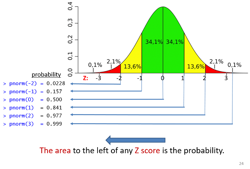
Once you have computed a Z-score, you can look up the probability in a table for the standard normal distribution or you can use the pnorm() function in R. The illustration below shows the probabilities that would be obtained for selected Z-scores. Keep in mind that the probabilities obtained from tables for the standard normal distribution or pnorm give the area (probability) to the left of that Z-score.
Computing Probabilities from the Standard Normal Distribution
pnorm(Z)
If you have compted a Z-score you can find the probability of a Z-score less than that by using pnorm(Z).
Suppose that BMI measures for men age 60 in the Framingham Heart Study population is normally distributed with a mean (μ) = 29 and standard deviation (σ) = 6. You are asked to compute the probability that a 60 year old man in thispopulation will have a BMI less than 30. First, you calculate the Z-score for a BMI of 30:

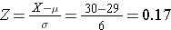
Next, you use R to compute the probability of a Z-score less than 0.17:
pnorm(0.17)
[1] 0.5674949
The probability that a 60 year old man in this population will have a BMI less than 30 is 56.7%.
pnorm(X, μ, SD)
Using the same problem as in the previous example, you can also use R to compute the probabilty directly without computing Z.
pnorm(30,29,6)
[1] 0.5661838
You can also calculate the probability that a 60 year old man in this population would have a BMI greater than 30 either from the Z-score or from the mean and standard deviation.
1-pnorm(0.17)
[1] 0.4325051
1-pnorm(30,29,6)
[1] 0.4338162
Thus, the probability that a 60 year old man will have a BMI greater than 30 is 43%.
We can also compute the probability that a 60 year old man in this population will have a BMI between 30 and 40.
pnorm(40,29,6)-pnorm(30,29,6)
[1] 0.4004397
The probability of BMI between 30 and 40 is 40%.
Computing Percentiles
When asked to compute a percentile, we are using similar information, but we are asked to compute the measure that corresponds to a given probability or percentile. For example, suppose we are still dealing with the same population of 60 year old men in the Framingham Study. The mean BMI is still 29, and the standard deviation is 6. We are asked what value of BMI is the 90th percentile. In other words, 90% of men will have a BMI below what value?
The equation for computing a Z-score is

Now we are trying to find the value of X that corresponds to a probabllity of 90%. We can start by finding the Z-score for a probabilty of 90%, and to do that we can use the R function shown below.
qnorm(p)
This gives the Z score associated with the standard normal probability p.
qnorm(0.90)
[1] 1.281552
Now we can plug the numbers into the equation.
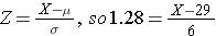
We now can rearrange the equation algebraically to solve for the value of Z.

Therefore, the 90th percentile for BMI is 36.7, meaning that 90% of 60 year old men in this population will have a BMI less than 36.7.
And we could have done this calculation directly in R as well using
qnorm(p, μ, σ) , where p is the desired percentile (probability), μ is the mean, and σ is the standard deviation as shown in the example below.
qnorm(0.9,29,6)
[1] 36.68931
This gives the same result. 90% of 60 year old men in this population will have a BMI less than 36.7