


Correlation and Simple Linear Regression
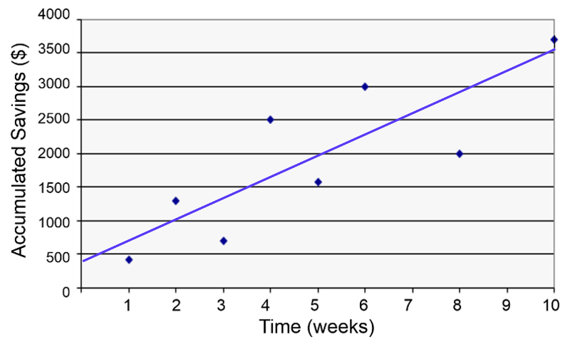
When looking for a potential association between two continuously distributed measurement variables, we can begin by creating a scatter plot to determine whether there is a reasonably linear relationship between them. The possible values of the exposure variable (i.e., predictor or independent variable) are shown on the horizontal axis (the X-axis), and possible values of the outcome (the dependent variable) are shown on the vertical axis (the Y-axis).
plot(Savings~Week)
You can add the regression line to the scatter plot with the abline() function.
abline(lm(Savings~Week))
The regression line is determined from a mathematic model that minimizes the distance between the observation points and the line. The correlation coefficient (r) indicates how closely the individual observation points conform to the regression line.
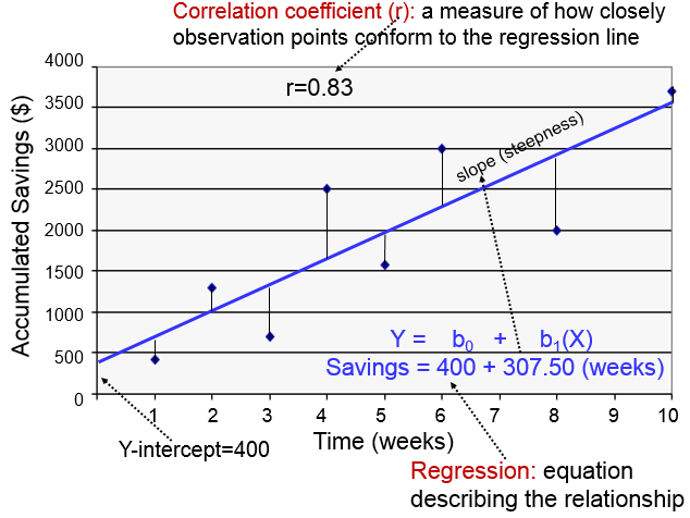
The steepness of the line is the slope, which is a measure of how many units the Y-variable changes for each increment in the X-variable; in this case the slope provides an estimate of the average weekly increase in savings. Finally, the Y-intercept is the value of Y when the X value is 0; one can think of this as a starting or basal value, but it is not always relevant. In this case, the Y-intercept is $400 suggesting that this individual had that much in savings at the beginning, but this may not be the case. She may have had nothing, but saved a little less than $500 after one week.
Notice also that with this kind of analysis the relationship between two measurement variables can be summarized with a simple linear regression equation, the general form of which is:

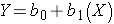
where b0 is the value of the Y-intercept and b1 is the slope or coefficient. From this model one can make predictions about accumulated savings at a particular point in time by specifying the time (X) that has elapsed. In this example, the equation describing the regression is:
SAVINGS=400 + 307.50 (weeks)
Correlation Coefficient
cor(xvar, yvar)
This calculates the correlation coefficient for two continuously distributed variables. You should not use this for categorical or dichotomous variables.
cor(hgt_inch,weight)
[1] 0.5767638
Correlation Coefficient and Test of Significance
cor.test(xvar, yvar)
This calculates the correlation coefficient and 95% confidence interval of the correlation coefficient and calculates the p-value for the alternative hypothesis that the correlation coefficient is not equal to 0.
cor.test(hgt_inch,weight)
Pearson's product-moment correlation
data: hgt_inch and weightt = 40.374, df = 3270, p-value < 2.2e-16
alternative hypothesis: true correlation is not equal to 095 percent confidence interval:
0.5534352 0.5991882sample estimates:
****cor
0.5767638
Simple Linear Regression
reg_output_name<-lm(yvar~xvar)
summary(reg_output_name)
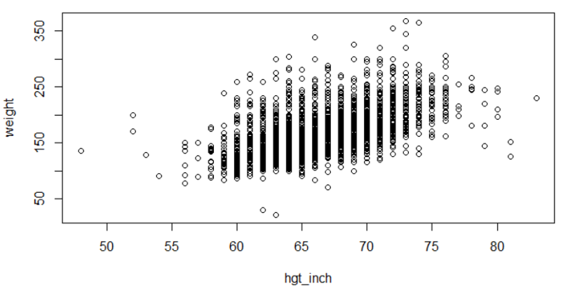
Linear regression in R is a two part command. The first command fits a linear regression line with yvar (outcome) and xvar (predictor) to the "reg_output_name" (you can use any name). The summary() command prints out the regression equation and summary statistics. Be sure to use the ~ character between the Y-variable (outcome) and the X-variable (predictor). Here is a simple linear regression of weight as a function of height from the Weymouth Health Survey.
plot(weight~hgt_inch)
myreg<-lm(weight~hgt_inch)
abline(myreg, col = 'red')
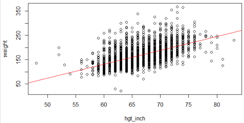
summary(myreg)
Call:
lm(formula = weight ~ hgt_inch)
Residuals:
*****Min *****1Q Median ****3Q ****Max
-127.413 -21.824 -4.837 15.897 172.451
Coefficients:
*************Estimate Std. Error t value Pr(>|t|)
(Intercept) -211.4321 ****9.4202 *-22.45 *<2e-16 ***
hgt_inch *******5.7118 ****0.141 ***40.37 *<2e-16 ***
---
Signif. codes: 0 '***' 0.001 '**' 0.01 '*' 0.05 '.' 0.1 ' ' 1
Residual standard error: 32.64 on 3270 degrees of freedom
Multiple R-squared: 0.3327, Adjusted R-squared: 0.3325
F-statistic: 1630 on 1 and 3270 DF, p-value: < 2.2e-16