R Programming for PH717
This module provides a summary of R commands and functions that are likely to be used in PH717. This module is not meant to be studied; it is a reference that enables you to look up how to perform a variety of procedures in R.
NOTE: The Contents link on the left side of each page takes you to a hyperlinked table of contents that will make it easy for you to find the specific task you are looking for.
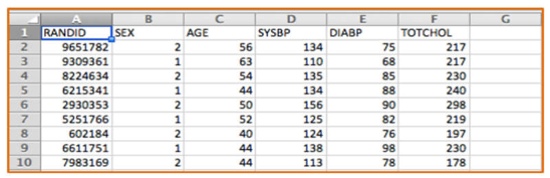
One can think of data sets series of tables with many variables (demographic information, exposures and outcomes) in the columns and each subject listed on a separate row. The figure below shows a portion of an Excel spreadsheet that was used to download the first 10 subjects in a very small subset of the Framingham Heart Study. There is a random identification number in the first column, and columns indicating each subject's sex, age in years, systolic blood pressure, and total cholesterol. There are many more variables, but this small subset gives you an idea of the structure of a data set.
Designating Dichhotomous Variables as True or False
Note that the variable SEX is coded as 1 or 2, and we would need a key to know which is for males and which is for females. A better way to do this for dichotomous variables is to give the variable a more explicit name such as "MALE" and use 1 to indicate "yes" or "true" and 0 to indicate "no" or "false". This will make subequent analysis easier and more explicit.
Excel spreadsheets can be used to collect and store tables of data of this type, and Excel can also be used for a variety of simple statistical tests. For example, Excel can perform chi-squared tests, t-tests, correlations, and simple linear regression. However, it has a number of limitations. Public health researchers and practitioners frequently perform more complex analyses, such as multiple linear regression and multiple logistic regression, which cannot be performed in Excel, so it is useful to become familiar with more sophisticated packages like R.
[NOTE: There is an online learning module on how to use Excel for public health at Using Spreadsheets - Excel & Numbers]
All data sets used in PH717 are comma separated value (.csv) files. These are like spreadsheets in that they contain rows and columns of alphanumeric data, but they have a much simpler format than true spreadsheets, which are .xlsx files. One can import .xlsx files into R, but in PH717, all of the data sets will be in .csv format.
Note also that one can create .csv files using Excel. One would open Excel and insert the data in rows and columns and then use "File", "Save as" to save the data as a .csv file.
You will first install the base system for R and then install the RStudio, which provides a much more user-friendly interface.
In your browser go to https://cran.r-project.org/
Select Download R for Mac or for Windows

In your browser go to https://www.rstudio.com/products/rstudio/

Once the RStudio is installed, it will have several windows as shown in the image below.

The modules for this course have many examples of how to use R for specific tasks, and you will be using these from week to week. The examples embedded into each week?s learning modules will provide you with all of the necessary instructions for using R in this course, and it shouldn't be necessary to seek other instruction. However, if you wish to learn more about R, here are links to additional resources.
The 10 minute video below walks you through using R Studio to import a data set, how to create and execute a script to analyze it, and how to create and export graphs..
THe "Console" window in R Studio can be used as a calculator.
For the examples below:
Try entering the following commands in the R Console at the lower left window. You do not have to enter the comments in green. Just enter the commands in blue and hit "Enter". You should see the result written in black after the [1].
# Addition
> 7+3
[1] 10
# Subtraction
> 7-3
[1] 4
# Multiplication
> 8*7
[1] 56
# Division
> 100/50
[1] 2
# Square root
> sqrt(81)
[1] 9
# Exponents
> 9^2
[1] 81
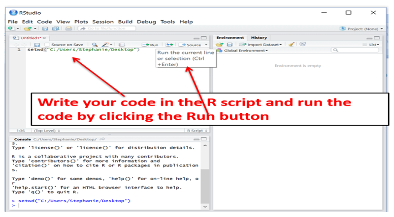
You can execute code one step at a time in the console (lower left window), and this is useful for quick one step math calculations, but it is usually more convenient to list all of your coding statements in a script in the window at the upper left and then saving the script for future use. When you enter code into the script window at the upper left, do not begin the line with a > character. You can also execute the code from the script editing window by clicking on the "Run" tab at the top of the editing window. To save a script, click on the "File" tab at the upper left and select either Save as or Save.
Data sets that are saved on your local computer can be imported into R. If the data set is posted on a website, first save it to your local computer and then import it.
The older method for importing data sets in to use the read.csv(file.choose()) command. If I were to enter the line of code below into the Console window at the lower right, without a file name in the inner parentheses and then hit the Enter key, it would open a dialog box that allowed me to locate the file on my local computer.
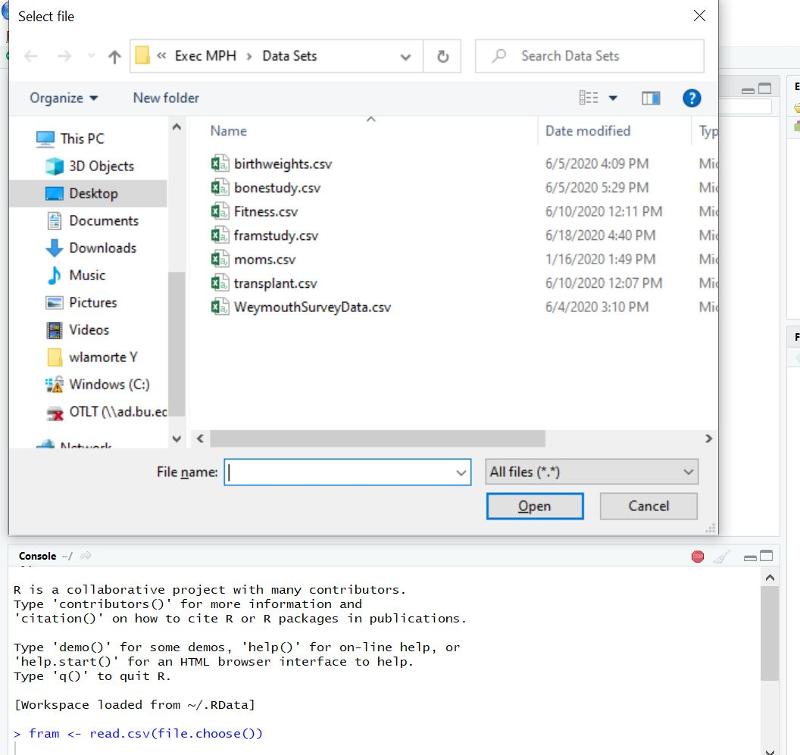
Note that the window may not fully open, but might appear on your taskbar at the bottom of your screen if you are using a PC (see the brown highlghted selection on my taskbar in the image below.

If you click on the highlighted selection on the taskbar, it will open the dialog box in the previous image, and you can browse to locate and select the data file.
Once you double click on the data file to select it, it will import the data set and give it the nickname "fram" in this case, a nickname that I chose just to allow less typing when referring to the data set. Then, to view the data set in the upper left window, you can use the command View(fram), noting that this particular commaned uses an uppercase "V", although most are lowercase.
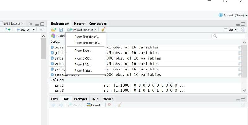
The easiest way is to click on the "Import Data set" button in the upper right window of R Studio. A pop-down menu will open. If you are importing a .CSV file, choose the first option (From text(base)).
This will open another window enabling you to browse your computer to locate the file you want to import. Double click on the file, and another window will open as shown below.
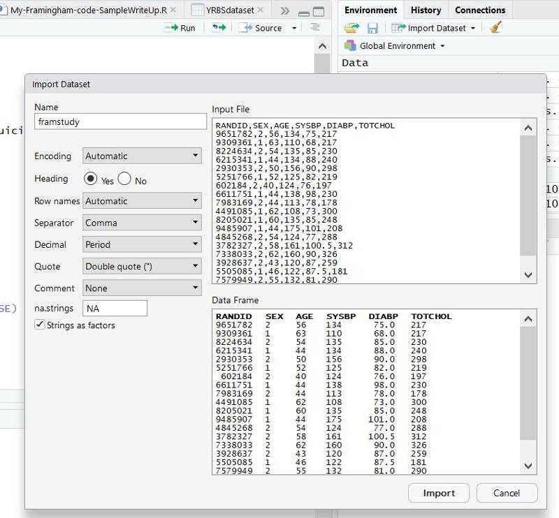
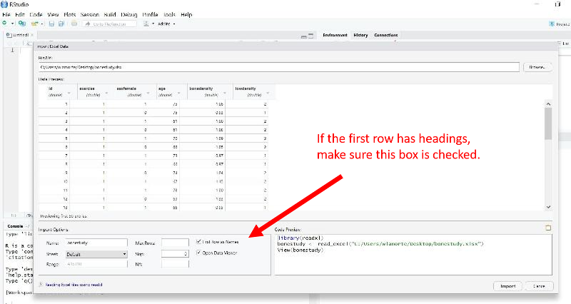
Does the Data Have Headings?
On the left side there is an option to indicate whether the data set has Headings (variable names at the top of the columns). All of the PH717 data sets have headings, so make sure "Yes" is selected. Then click on the "Import" button at the bottom of this window.
When the data is imported, R should show the data in the upper left window of the R Studio, and you can scroll right and left and up and down to check the data set for errors. Notice also that R has created a tab just below the main menu with the title for the data set (framstudy in this case).
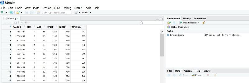
The data set is also now listed in the window at the upper right and indicates that it has 49 observations and 6 variables.
You can review the data set at any time by clicking on the tab with its name in the upper left window or by clicking on the data set name in the upper right window. You can also review it using the "View()" command in R, e.g., View(framstudy) and then hitting the "Run" button in the upper left window. Note that this R command uses an uppercase "V", although most commands use lower case.
All of the data sets for PH717 are .CSV files, but you can import data from .XLSX files. Once again, use the "Import Dataset" button in the upper right window in R Studio, but select the third option (From Excel).
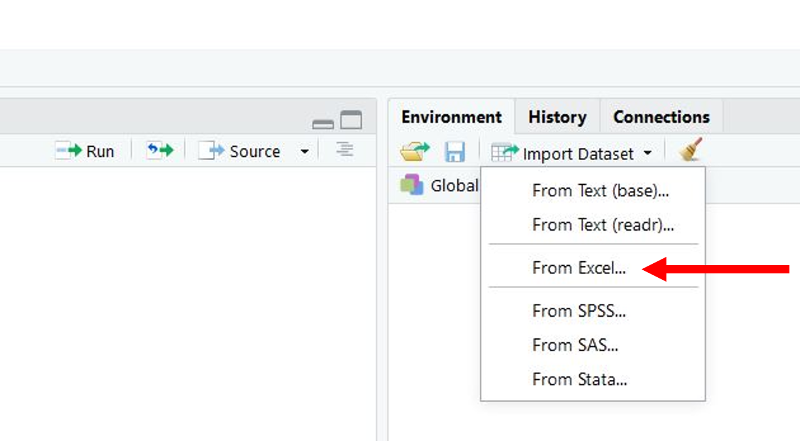
This will open a window that enables you to browse for the data file you want. Once you locate it, click to select it and then click on the "Import" button at the bottom.
A script in R is a series of commands and function instructing R how to analyze the data. A script can be save and retrieved later for corrections or modifications.
You can execute code one step at a time in the R Studio Console (lower left window), and this is useful for quick one step math calculations, but if you have a sequence of coding statement, it is more convenient to list all of your coding statements in a script in the window at the upper left and then saving the script for future use. Note that when you enter code into the script window at the upper left, do not begin the line with a > character.
Writing Code in R - Important Notes
Nicknaming Your Data Set, Attaching, and Detaching It
You can give the data set a nickname to reduce typing. For example, if I imported a data set called framstudy, I might nickname it "fram" to reduce typing by including this command after the data is imported:
fram<- framstudy
Once the data set has been imported, you should "attach" the data so that R defaults to performing actions on this particular data set.
attach(fram)
If you finish with an attached data set and want to work with another data set, you should detach the first one > detach(fram)] and then import and attach the new one.
Here is an example showing the first part of a script in the upper left window of R Studio.
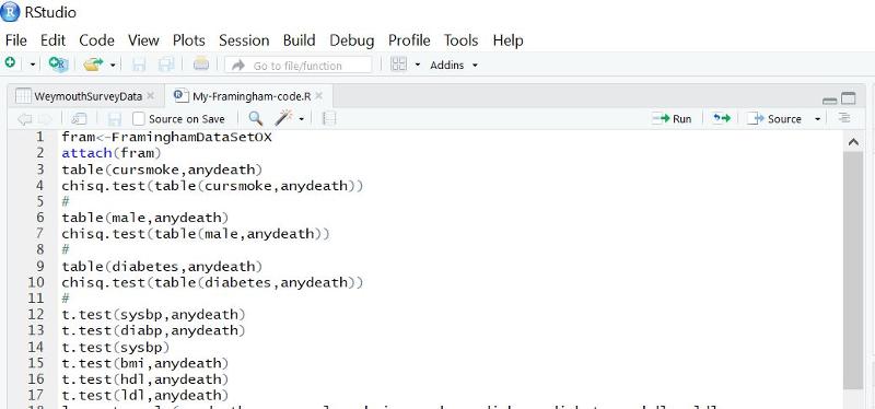
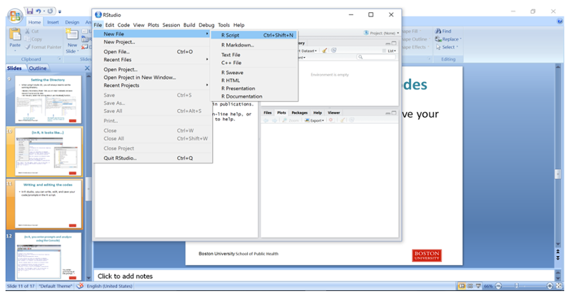
To start a new script, click on the File tab, then on New File, then on R Script.
Then type in your coding statements.
Here is a short sample script:
The line that says attach(fram)attaches the data set, basically telling R that subsequent data steps should be executed on this particular data set. At the end of the script, one can use the command detach(fram) to detach it.
# (A comment) Import the framstudy.csv file and call it "fram"
########################
fram<- framstudy # Next attach the file to tell R it is the "go to" file (the default)
attach(fram)
View(fram)
# Determine the mean, median, and distribution of continuous variables
quantile(AGE)
summary(AGE)
# Determine the number and proportion of males and females
table(SEX)
prop.table(table(SEX))
# Make a mistake in case
summary(Age)
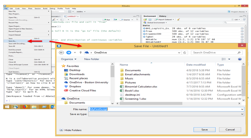
Enter the script above into the R editor and save it as follows:
Then execute the script by hitting the "Run" tab repeatedly in the editor. When you get to the "View(fram)" step, the editor will show the data file, but you can return to the script by clicking on the tab for the script at the top of the window.
The output from the executed script will appear in the Console window at the lower left, and it should look like this:
fram<- framstudy
attach(fram)
View(fram)
quantile(AGE)
0% *25% 50% 75% 100%
39 45 *52 *59 **65
summary(AGE)
*Min. 1st Qu. Median *Mean 3rd Qu. Max.
39.00 **45.00 *52.00 52.41 *59.00 65.00
table(SEX)
SEX
*1 *2
19 30
prop.table(table(SEX))
SEX
********1 ********2
0.3877551 0.6122449
summary(Age)
Error in summary(Age) : object 'Age' not found
Note that there was an error message because we gave the command "summary(Age)", but the variable for age is all upper case (AGE), so R did not find it.
Also note that you can copy the commands and resulting output from the Console and paste them into other applications, such as Word files.
Suppose I have data from a survey that was conducted in 2002 in which one of the variables is birth_yr, i.e., the year in which the subject was born. I want to create a variable called "age" that shows how old the subject were at the time the survey was conducted. To do this I can create a derived variable as follows in one of my script lines:
# Create a derived variable for the respondent's age in 2002 (when the data was collected) based on their reported birth year.
age=(2002-birth_yr)
Suppose the data set also has a column for the subject's height in inches (hgt_inch) and weight in pounds (weight), but I want to compute each subject's body mass index (bmi). There is a formula for computing bmi from height in inches and weight in pounds, and I can compute bmi by including a line of code in my script.
# Compute body mass index (bmi)
bmi=weight/(hgt_inch)^2*703
This divides weight in pounds by height in inches squared times 703.
Body mass index is a continuous distributed variable, i.e., it can have an infinite number of values within a certain range. However, suppose I also wanted to categoize subjects as to whether they were obese (bmi of 30 or more) versus non-obese (bmi<30). I can use the ifelse() function in R to create a new variable called "obese" with a value of 1 if bmi is greater than or equal to 30 and a value of 0 if bmi is less than 30.
ifelse(conditional statement, result if true, result if false)
For each subject the conditional statement is evaluated to determine if it is true for that subject or not. If it is true, R assigns the next value to the new variable; if it is false, it assigns the second value to the new variable.
The first line of code below is a conditional statement that creates a new variable called "obese". It says to evaluate each subject's bmi, and, if it is less than 30, assign a value of 0 to obese (meaning that the individual is not obese). If that condition is not met, i.e. if the value of bmi is greater than or equal to 30, obese will have a value of 1, meaning that the individual is in the obese category.
obese=ifelse(bmi<30,0,1)
I can then include a line of code that asks R to give a tabulation of the variable obese.
table(obese)
The output:in the Console indicates that there were 3272 subjects, and onlky 3 of them were in the obese category.
**obese
*****0 1
3269 3
One of the surveys conducted by the Youth Behavior Risk Surveillance System (YRBSS) had variables that reflected student response to two questions about bullying and three questions about suicide.
|
Variable Name |
Quesion and Coding |
|---|---|
|
bully.sch |
During the past 12 months, have you been bullied on school property? 1=yes 0=no |
|
bully.online |
During the past 12 months, have you been electronically bullied (e-mail, chat rooms, instant messaging, Web sites, or texting)? 1=yes 0=no |
|
suicide.consider |
During the past 12 months, did you ever seriously consider attempting suicide? 1=yes, 0=no |
|
suicide.plan |
During the past 12 months, did you make a plan about attempting suicide? 1=yes 0=no |
|
suicide.attempt |
During the past 12 months, did you actually attempt suicide? 1=yes 0=no |
For part of my analysis I want to examine whether any form of bullying (in school or online) was associated with any indications of suicide risk (i.e., considering, planning or attempting suicide).
I can collapse the two questions about bullying into a single variable I will call "anyB", meaning any form of bullying, and I can collapse the three questions about suicide into a single variable I will call "anyS", i.e., whether there was any indication of suicide risk. I will use two conditional statements to do this.
anyB<-ifelse(bully.sch+bully.online>0,1,0)
This adds the variables for bull.sch and bully.online. If both are positive responses, the result is 2; if one or the other is positive, the result is 1; if neither is positive, the result is 0. The conditional statement evaluates the sum of the two variables, and if the sum is greater than 0, it gives anyB a value of 1, meaning true. If neither form of bullying occurred, the sum will be 0, and R will give anyB a value of 0.
Similarly, I can create a new variable called "anyS", indicating whether the subject gave any responses indicating risk of suicide.
anyS<-ifelse(suicide.consider+suicide.plan+suicide.attempt>0,1,0)
This evaluates the sum of the three variables indicating some risk of suicide. If the sum is 0, anyS is assigned a value of 0, but if one or more of the three suicide indicators is true, then anyS is assigned a value of 1.
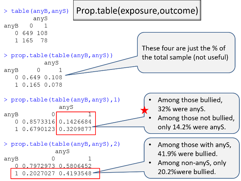
Having done this, I can then use the table() command to generate a contingency table for the association between anyB and anyS.
table(anyB,anyS)
****anyS
anyB 0 1
0 *649 **108
1 *165 78
summary(varname)
Provides minimum, 1st quartile (25%tile), median, mean, 3rd quartile (75%tile) and maximum values of varname.
summary(age)
**Min. 1st Qu. Median *Mean 3rd Qu. *Max.
61.00 **63.00 *66.00 *66.94 **70.00 75.00
mean(varname)
mean(age)
[1] 66.94286
sd(varname)
sd(age)
[1] 4.458586
median(varname)
median(age)
[1] 66
To compute descriptive statistics for continuous variables by group, use the tapply() function
tapply(varname, groupname, statistic)
Provides statistics for varname by groupname. Statistics can be summary, mean, sd and others.
tapply(bmi,anyS,mean)
This gives the mean of bmi separately for those with variable anyS=0 and anyS=1.
***0 1
23.4358 23.6796
Similarly, we can compute the standard deviation for bmi in each of these two groups.
tapply(bmi,anyS,sd)
**0 1
4.971052 4.665697
table(varname)
Provides frequency counts for each value of varname.
Here is a simple 2x2 table showing the number of students reporting suicidal risk in obese (bmi>30) and non-obese students.
table(obese,anyS)
****anyS
obese 0 1
0 704 **159
1 110 *27
Here is a 4x2 table reporting the counts of anyS by grade in high school.
table(grade,anyS)
anyS
grade
******0 **1
9 ***193 50
10 ***192 57
11 ***228 46
12 ***201 33
prop.table(table(varname))
This gives the proportion for each value of varname. There are three variation of this, depending on whether you want the proportions by row, by column, or overall as illustrated in the examples below..
prop.table(table(lowdensity,exercise))
exercise
lowdensity
**********0 ********1
1 0.2857143 0.1142857
2 0.2857143 0.3142857
These four proportions add up to 1.0, i.e., each is the proportion based on the total number of observations
prop.table(table(lowdensity,exercise),1)
exercise
*******lowdensity
**********0 ********1
1 0.7142857 0.2857143
2 0.4761905 0.5238095
This table gives the proportions across rows, i.e., the proportions are for the total number in each row, and the proportions for each row add up to 1.0.
prop.table(table(lowdensity,exercise),2)
exercise
********lowdensity
**********0 ********1
1 0.5000000 0.2666667
2 0.5000000 0.7333333
This table gives the proportions across columns, i.e., the proportions are for the total number in each column, and the proportions in each column add up to1.0.
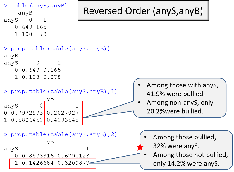
Example: I am conducting a case-control study in which the primary exposure of interest is being bullied (anyB), and the outcome of interest is any indication of suicidal risk (anyS). I want to make a table that compares exposure frequency in the cases and controls. I can use the table() command to get the counts, and I can use the prop.table() command to get the proportions. However, I need to think about a) the order of the variables and b) the "flag" that I use in the prop.table() command.
In the sequence of R output on the left, the epression in parenthesis has the exposure, then the outcome. If no flag is used in prop.table, R gives the proportion in each cell relative to the total sample, which is not helpful. If I add the ",1" flag, I get the desired output, the proportion with the outcome in each exposure group.
In the sequence on the right, however, it is the ",2" flag in prop.table that provides the proportion with the outcome in each exposure group.
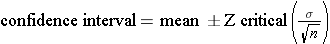
A Z score represents how many standard deviations an observation is away from the mean. The mean of the standard normal distribution is 0. Z scores above the mean are positive and Z scores below the mean are negative.
Once you have computed a Z-score, you can look up the probability in a table for the standard normal distribution or you can use the pnorm() function in R. The illustration below shows the probabilities that would be obtained for selected Z-scores. Keep in mind that the probabilities obtained from tables for the standard normal distribution or pnorm give the area (probability) to the left of that Z-score.
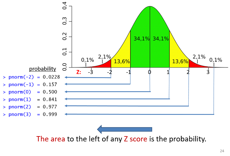
If you have compted a Z-score you can find the probability of a Z-score less than that by using pnorm(Z).
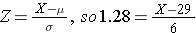
Suppose that BMI measures for men age 60 in the Framingham Heart Study population is normally distributed with a mean (μ) = 29 and standard deviation (σ) = 6. You are asked to compute the probability that a 60 year old man in thispopulation will have a BMI less than 30. First, you calculate the Z-score for a BMI of 30:
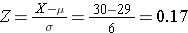
Next, you use R to compute the probability of a Z-score less than 0.17:
pnorm(0.17)
[1] 0.5674949
The probability that a 60 year old man in this population will have a BMI less than 30 is 56.7%.
Using the same problem as in the previous example, you can also use R to compute the probabilty directly without computing Z.
pnorm(30,29,6)
[1] 0.5661838
You can also calculate the probability that a 60 year old man in this population would have a BMI greater than 30 either from the Z-score or from the mean and standard deviation.
1-pnorm(0.17)
[1] 0.4325051
1-pnorm(30,29,6)
[1] 0.4338162
Thus, the probability that a 60 year old man will have a BMI greater than 30 is 43%.
We can also compute the probability that a 60 year old man in this population will have a BMI between 30 and 40.
pnorm(40,29,6)-pnorm(30,29,6)
[1] 0.4004397
The probability of BMI between 30 and 40 is 40%.
When asked to compute a percentile, we are using similar information, but we are asked to compute the measure that corresponds to a given probability or percentile. For example, suppose we are still dealing with the same population of 60 year old men in the Framingham Study. The mean BMI is still 29, and the standard deviation is 6. We are asked what value of BMI is the 90th percentile. In other words, 90% of men will have a BMI below what value?
The equation for computing a Z-score is

Now we are trying to find the value of X that corresponds to a probabllity of 90%. We can start by finding the Z-score for a probabilty of 90%, and to do that we can use the R function shown below.
qnorm(p)
This gives the Z score associated with the standard normal probability p.
qnorm(0.90)
[1] 1.281552
Now we can plug the numbers into the equation.
We now can rearrange the equation algebraically to solve for the value of Z.

Therefore, the 90th percentile for BMI is 36.7, meaning that 90% of 60 year old men in this population will have a BMI less than 36.7.
And we could have done this calculation directly in R as well using
qnorm(p, μ, σ) , where p is the desired percentile (probability), μ is the mean, and σ is the standard deviation as shown in the example below.
qnorm(0.9,29,6)
[1] 36.68931
This gives the same result. 90% of 60 year old men in this population will have a BMI less than 36.7
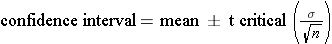
The T-distribution is similar to the standard normal distribution, but it doesn't assume that the sample size is large. It is particularly useful for small samples because it is really a series of distributions that adjust for sample size by taking into account the degrees of freedom. R often defaults to using the t-distribution, because it can be used for both small and large samples. When the sample size is large, the t-distribution is very similar to the standard normal distribution.
pt(t, df)
This gives the probability corresponding to a t-statistic and a specified number of degrees of freedom, i.e., P(tdf < t)
qt(p, df)
This gives the critical value to the t-distribution associated with the probability p and df (degrees of freedom)= n-1. It answers the question, what is the critical t-statistic for a given probability and specified degrees of freedom, i.e., what is the minimum value of t for a specified probabilty and a specifed degrees of freedom.
Previously, we used Z-scores to compute that probability that an individual in a population with known mean and standard deviation would have a measurement (e.g., BMI) less than or greater than a certain value. However, this method addresses a different question: what is the probability that a sample mean will have a value less than or greater than a certain value. To illustrate, we can once again use the population of 60-year old men in the Framingham cohort.
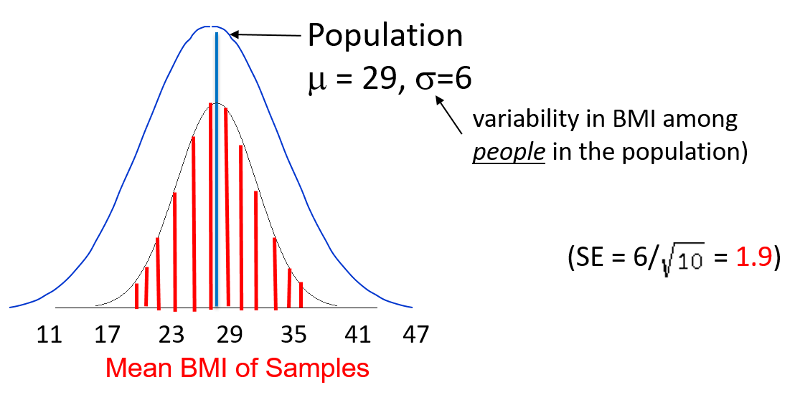
If you recall, the population had a mean BMI of 29 with a standard deviation of 6. Now that we are addressing a sample mean rather than an individual, we need to use the standared error instead of the standard deviation. In this case, the standard error is 1.9, as shown above.
Question: Given this scenario, what is the probability of taking a sample from the population and finding a sample mean less than 23?
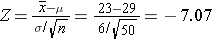
pnorm(-7.07)
[1] 7.746685e-13
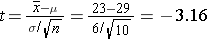
pt(-3.16,9)
[1] 0.005775109
Even with the smaller sample, the probability of a sample mean less than 23 is very small, but no where near a small as that obtained with a larger sample using the standard normal disttribution.
A study measured the verbal IQ of children in 30 children who had been anemic during infancy. The mean was 101.4 and the standard deviation was 13.2. What was the 95% confidence interval for the estimated mean?
For a 95% confidence interval Zcritical = 1.96.
 with n-1 degrees of freedom
The problem states a sample size of 30, so we will use use t-critical with 30-1=29 degrees of freedom. A 95% confidence interval would encompass all but the bottom 2.5% and the top 97.5% which correspond to probabilities of 0.025 and 0.975. We can use qt(p,df)to compute the critical value of t.
qt(0.975,29)
[1] 2.04523
qt(0.025,29)
[1] -2.04523
Therefore, the critical value of t is about 2.05. We can now compute the 95% confidence interval:
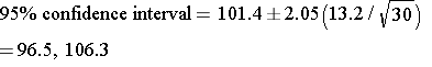
With 95% confidence, the true mean lies between 96.5 and 106.3.
The confidence interval for a mean is even simpler if you have a raw data set and use R, as shown in this example.
t.test(age)
One Sample t-test
data: age
t = 88.826, df = 34, p-value < 2.2e-16
alternative hypothesis: true mean is not equal to 0
95 percent confidence interval:
65.41128 68.47444
sample estimates:
mean of x
*****66.94286
Here the mean is 66.9. With 95% confidence the true mean lies is between 65.4 and 68.5.
You can use tapply()
tapply(varname, groupname, t.test)
tapply(bonedensity,exercise,t.test)
# First is reports on non-exercisers,i.e. exercise=0
$`0`
One Sample t-test
data: X[[i]]
t = 28.088, df = 19, p-value < 2.2e-16
alternative hypothesis: true mean is not equal to 0
95 percent confidence interval:
0.913452 1.060548
sample estimates:
mean of x
**********0.987
# Then it reports on exercisers,i.e. exercise=1
$`1`
One Sample t-test
data: X[[i]]
t = 33.123, df = 14, p-value = 1.062e-14
alternative hypothesis: true mean is not equal to 0
95 percent confidence interval:
1.020043 1.161290
sample estimates:
mean of x
**********1.090667
prop.test(numerator, denominator, correct=FALSE)
If the sample size is greater than 30, use correct=FALSE. If the sample size is less, use correct=TRUE.
prop.test(1219,3532,correct=FALSE)
1-sample proportions test without continuity correction
data: 1219 out of 3532, null probability 0.5
X-squared = 338.855, df = 1, p-value < 2.2e-16
alternative hypothesis: true p is not equal to 0.5
95 percent confidence interval:
0.3296275 0.3609695
sample estimates:
p
*****0.3451302
Interpretation: The point estimate for the proportion is 0.345. With 95% confidence, the true proportion is between 0.33 and 0.36.
This is used when a single sample is compared to a "usual" or historic population mean.
t.test(varname, μ =population mean)
Example: The mean IQ in the population=100. Do children who were born prematurely have lower IQ? Investigators measured the IQ of n=100 children who had been born prematurely. The mean IQ in this sample was 95.8 with a standard deviation (SD) of 17.5. What is the probability that a sample of 100 will have a mean IQ of 95.8 (or less)?
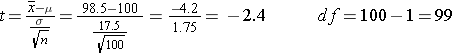
pt(-2.4,99)
[1] 0.009132283
However, this can be done completely with R if you have the raw data set.
t.test(iq,mu=100)
One Sample t-test
data: iq
t = -2.3801, df = 99, p-value = 0.01922
alternative hypothesis: true mean is not equal to 100
95 percent confidence interval:
92.35365 99.30635
sample estimates:
mean of x
95.83
In most cases, it is appropriate to do a two-tailed test for which the alternative hypothesis is that there is a difference without specifying which group is expected to be greater. However, there are situations for which a one-tailed test is accepable. If no option is specified, R will automatically perform the more conservative two-tailed comparison, but you can specify a one-tailed test.
In the example below, we test the null hypothesis that the bonedensity in a sample of people is not equal to one. In the first comparison, we do not specify whether to do a one-tailed or two-tailed test, so R automatically performs a two-tailed test.
t.test(bonedensity,mu=1)
One Sample t-test
data: bonedensity
t = 1.2205, df = 34, p-value = 0.2307
alternative hypothesis: true mean is not equal to 1
95 percent confidence interval:
0.9790988 1.0837583
sample estimates:
mean of x
1.031429
The difference was not statistically significant (p=0.23).
Next, the test is repeated as a one-tailed test specifying that we expect the sample to have a mean bonedensity greater than 1.
t.test(bonedensity,mu=1, alternative="greater")
One Sample t-test
data: bonedensity
t = 1.2205, df = 34, p-value = 0.1153
alternative hypothesis: true mean is greater than 1
95 percent confidence interval:
0.9878877 Inf
sample estimates:
mean of x
1.031429
The difference is once again not statistically significant (p=0.1153), but note that the p-value is half of that obtained with the more conservative two-tailed test.
If your alternative hypothesis is that the mean bonedensity for the sample is less than 1, you would use the following code:
t.test(bonedensity,mu=1, alternative="less")
This is used to compare means between two independent samples. This test would be appropriate if you were comparing means in two different groups of people in a clinical trial when the two groups were randomly allocated to receive different treatments.
There are two options for this test - one when the variances of the two groups are approximately equal and another when they are not. The variance is the square of the standard deviation.
To determine whether the variances for the two samples are reasonably similar, compute the ratio of the sample variances.
t.test(varname ~ groupname, var.equal=TRUE)
t.test(varname ~ groupname, var.equal=FALSE)
Example: I want to compare mean bonedensity measures in subjects who exercise regularly and those who do not.
# First I use tapply() to get the two standard deviations
tapply(bonedensity,exercise,sd)
0 1
0.1571489 0.1275296
# Then I find the ratio of the squared standard deviations
0.157^2/0.1286^2
[1] 1.49045
# The ratio is between 0.5 and 2.0, so I can use the equal variance option
# If you do not specify the var.equal option, it will assume they are unequal
t.test(bonedensity~exercise,var.equal=TRUE)
Two Sample t-test
data: bonedensity by exercise
t = -2.0885, df = 33, p-value = 0.04455
alternative hypothesis: true difference in means is not equal to 0
95 percent confidence interval:
-0.204653969 -0.002679364
sample estimates:
mean in group 0 mean in group 1
0.987000 1.090667
IMPORTANT NOTE!
When performing a t-test for independent groups, be sure to separate the variables with the ~ character. Do not separate them with a comma.
Below is en ecample of the correct way and the incorrect way using the same data set.
Correct Way:
> t.test(height~anyS,var.equal = TRUE)
Two Sample t-test
data: height by anyS t = 3.3696, df = 998, p-value = 0.0007816
alternative hypothesis: true difference in means is not equal to 0 95 percent confidence interval:
0.01217630 0.04613444
sample estimates:
mean in group 0 mean in group 1
1.694263 1.665108
Incorrect Way:
> t.test(height,anyS,var.equal = TRUE)
Two Sample t-test
data: height and anyS t = 117.71, df = 1998, p-value < 2.2e-16
alternative hypothesis: true difference in means is not equal to 0 95 percent confidence interval:
1.477801 1.527879
sample estimates:
mean of x mean of y 1.68884 0.18600
Note that the second method is comparing the mean height to the mean value of the dichotomous group variable, which makes no sense. It is giving an incorrect t-statistic, incorrect degrees of freedom, and an incorrect p-value.
t.test(varname1, varname2,paired=TRUE)
This is used for comparing the means of paired or matched samples, such as the following:
Example: Early in the HIV epidemic, there was poor knowledge of HIV transmission risks among health care staff. A training was developed to improve knowledge and attitudes around HIV disease. All subjects were given a test to assess their knowledge before the training and again several weeks after the training. The table below shows their scores before (Kscore1) and after the training (Kscore2).
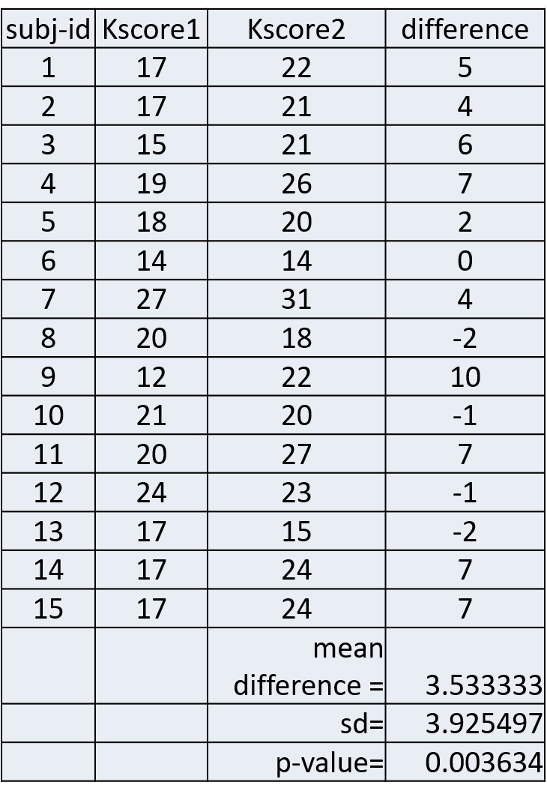
The column on the far right shows the difference in score for each subject and the mean differenence was 3.53333. The null hypothesis is that the mean difference is 0. Is there sufficient evidence to reject the null hypothesis and accept the alternative hypothesis that the before and after scores differed significantly?
This was tested using R as shown below.
# First the means scores before and after the test were calculated
mean(Kscore1)
[1] 18.33333
mean(Kscore2)
[1] 21.86667
# Then a paired t-test was performed
t.test(Kscore2,Kscore1,paired=TRUE)
Paired t-test
data: Kscore2 and Kscore1
t = 3.4861, df = 14, p-value = 0.003634
alternative hypothesis: true difference in means is not equal to 0
95 percent confidence interval:
1.359466 5.707201
sample estimates:
mean of the differences
3.533333
Interpretation: The mean difference was 3.533333. The confidence interval for the mean difference is from 1.36 to 5.71. We can conclude that on average, test scores improved 3.5 points after the training. With 95% confidence, the true mean improvement in scores was between 1.36 and 5.71 points.
chisq.test(varname1, varname2, correct = FALSE)
chisq.test(table(varname1, varname2), correct = FALSE)
Performs chi-square test on a contingency table. Use the correct=FALSE option with reasonably large sample sizes, ie., if expected counts in any of the cells in the contingency table have more than 5 observations. Use the correct = TRUE option, if expected counts in any cell in the contingency table are less than 5. When the correct=TRUE option is used, R performs the chi-squared test with Yates' continuity correction. If neither option is specified, R will perform the Yates correction automatically.
If you are working with a raw data set, the simplest way to do a chi-squared test is to use the first equation above. If I am working with the Weymouth Heatlh Survey data set, and I want to conduct a chi-squared test to determine whether there was an association between having a history of diabetes (hx_mi) and having had a myocardial infarction, i.e., a heart attack (hx_mi), I can use the following line of code:
chisq.test(hx_dm,hx_mi, correct=FALSE)
Pearson's Chi-squared test
data: hx_dm and hx_mi
X-squared = 132.67, df = 1, p-value < 2.2e-16
The output provides the chi-squared statistic, the degrees of freedom (df=1) and the p-value (2.2x10⁻¹⁶). When this line of code is run, R creates the contingency table in the background and then does the chi-squared test.
I can also do the chi-squared test from a contingency table that has already been created using the table() command.
table(hx_dm,hx_mi)
***hx_mi
hx_dm 0 1
0 *2832 142
1 **233 *65
chisq.test(table(hx_dm,hx_mi), correct=FALSE)
Pearson's Chi-squared test
data: table(hx_dm, hx_mi)
X-squared = 132.67, df = 1, p-value < 2.2e-16
Notice that this method gives the same results as the first method.
Suppose you don't have the raw data set. Instead, you are given the counts in a contingency table like this. This table summarizes whether HIV positive individuals disclosed their HIV status to their partners, and the the rows indicate how the subject had become infected with HIV.
|
Transmission |
Disclosure |
No Disclosure |
|
Intravenous drug use Gay contact Heterosex. contact |
35 13 29 |
17 12 21 |
Since we do not have access to the raw data, we need to construct the contingency table in R using a matrix() command. First, we create a contingency table, which I have arbitrarily named "datatable", and I give the command "datatable" so R will show me the table so I can check for errors.
datatable <- matrix(c(35,13,29,17,12,21),nrow=3,ncol=2)
datatable
[,1] [,2]
[1,] 35 17
[2,] 13 12
[3,] 29 21
This agrees with the counts that I started with, so I can go ahead and run the chi-squared test by simply referring to the name I gave to the contingency table and indicating that correct=FALSE, since the expected counts in all cells under the null hypothesis would be great than or equal to 5.
chisq.test(datatable,correct=FALSE)
Pearson's Chi-squared test
data: datatable
X-squared = 1.8963, df = 2, p-value = 0.3875
1-pchisq(chi-squared, df)
If you have a chi-squared statistic and the number of degrees of freedom (df), you can compute the p-value using the pchisq() command in R. However, the p-value is the area to the right of the chi-squared distributions, and pchisq() gives the area to the left. Therefore you have to subtract the pchisq() result from 1 to get the correct p-value.
Suppose a report you are reading indicates that the chi-squared value was 11.11 and there was 1 degree of freedom (df). The p-value would be computed as follows:
1-pchisq(11.11,1)
[1] 0.0008586349
riskratio.wald(exposure_var, outcome_var)
When dealing with a cohort study or a clinical trial, this command calculates a risk ratio and 95% confidence interval for the risk ratio and also performs a chi-squared test.
oddsatio.wald(exposure_var, outcome_var)
When dealing with a case-control study, this command calculates an odds ratio and 95% confidence interval for the odds ratio and also performs a chi-squared test.
Note: The "base package" in R does not have this function, but R has supplemental packages that can be loaded to add additional analytical tools, including confidence intervals for RR and OR. These tools are in the "epitools" package. You need to install the Epitools package into your version of R once from the Console in R Studio. Then, whenever you want to use the "wald" functions, you need to include a line in your script that will load the package.
Go to the Console window (lower left) in R and type:
>install.packages("epitools")
Be sure to include the quotation marks around "epitools". R wil install the package and display the following:
Installing package into 'C:/Users/wlamorte/Documents/R/win-library/3.5' (as 'lib' is unspecified) trying URL 'https://cran.rstudio.com/bin/windows/contrib/3.5/epitools_0.5-10.1.zip' Content type 'application/zip' length 317397 bytes (309 KB)
You only have to install the epitools package once, but you have to load it up each time you use it by including the following line of code in your script before the riskratio.wald command.
library(epitools)
R responds with:
Warning message: package 'epitools' was built under R version 3.4.2
I have a data set from the Framingham Heart Study, and I want to compute the risk ratio for the association between type 2 diabetes ("diabetes") and risk of being hospitalized with a myocardial infarction ("hospmi"). I begin by creating a contingency table with the table() command.
table(diabetes,hospmi)
************hospmi
diabetes 0 1
*******0 2557 210
*******1 183 48
Then, to compute the risk ratio and confidence limits, I insert the table parameters into the riskratio.wald() function:
riskratio.wald(table(diabetes,hospmi))
$data
**************hospmi
diabetes ***0 1 Total
*******0 2557 210 2767
*******1 183 48 231
Total ***2740 258 2998
$measure
risk ratio with 95% C.I.
diabetes estimate lower upper
*******0 1.00000 NA NA
*******1 *2.73791 2.062282 3.63488
NOTE: I changed the text color to red to call it to your attention. R does not do this.
Using the same data for illustration, I can similarly compute an odds ratio and its confidence interval using the oddsratio.wald() function:
oddsratio.wald(table(diabetes,hospmi))
$data
hospmi
diabetes **0 1 Total
*******0 2557 210 2767
*******1 183 48 231
***Total ***2740 258 2998
$measure
odds ratio with 95% C.I.
diabetes estimate lower upper
*******0 1.000000 NA NA
*******1 *3.193755 2.256038 4.521233
There are many extra packages for R and many alternate ways to compute things. Another package that is useful for risk ratios and odds ratios is the epiR package. Like the epi.tools package, it must be installed once, and then it must be loaded into each script in which it is used.
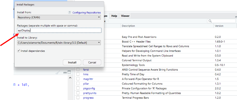
To do the one time installation, go to the lower right window and click on the Packages tab and then on the Install tab. In the window that opens, enter epiR as shown below.
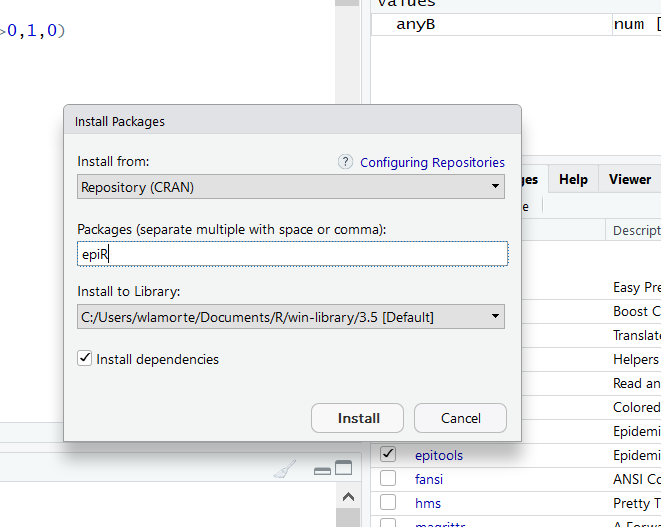
Then click on the Install button, and wait a few seconds while the package is installed.
Then, to use the program, you must load it into your script. Here is an example of its use in calculating a risk ratio, the 95% confidence interval for the risk ratio, the risk difference, and the attributable fraction.
In the example below, I use a data set from the Framingham Heart Study to create a table called "TAB" that summarizes the occurrence of being hospitalized for a myocardial infarction (hospmi) for diabetics and non-diabetics. I then print TAB to verify the counts, then call up the epiR package, and then give the command
> epi.2by2(TAB,method="cohort.count", conf.level = 0.95)
This asks R to use the data object called "TAB" and to analyze it as counts in a cohort study and compute the 95% confidence interval for the risk ratio.
> TAB<-table(diabetes, hospmi)
> TAB
hospmi
diabetes 0 1
0 2557 210
1 183 48
> library(epiR)
Package epiR 1.0-15 is loaded
Type help(epi.about) for summary information
Type browseVignettes(package = 'epiR') to learn how to use epiR for applied epidemiological analyses
> epi.2by2(TAB,method="cohort.count", conf.level = 0.95)
Outcome + Outcome - Total Inc risk * Odds
Exposed + 2557 210 2767 92.4 12.18
Exposed - 183 48 231 79.2 3.81
Total 2740 258 2998 91.4 10.62
Point estimates and 95% CIs:
-------------------------------------------------------------------
Inc risk ratio 1.17 (1.09, 1.25)
Odds ratio 3.19 (2.26, 4.52)
Attrib risk * 13.19 (7.87, 18.51)
Attrib risk in population * 12.17 (6.85, 17.50)
Attrib fraction in exposed (%) 14.27 (8.34, 19.82)
Attrib fraction in population (%) 13.32 (7.73, 18.57)
-------------------------------------------------------------------
Test that OR = 1: chi2(1) = 47.158 Pr>chi2 = <0.001
Wald confidence limits
CI: confidence interval
* Outcomes per 100 population units
NOTE: The "Attributable Risk (Attrib risk;) is the risk difference. The last two measures can be ignored for PH717. Also, since the Framingham Heart Study was a cohort study, we can ignore the odds ratio.
If we were analyzying a table from a case control study, we would use the following command:
> epi.2by2(TAB, method="case.control", conf.level = 0.95)
Outcome + Outcome - Total Prevalence * Odds
Exposed + 2557 210 2767 92.4 12.18
Exposed - 183 48 231 79.2 3.81
Total 2740 258 2998 91.4 10.62
Point estimates and 95% CIs:
-------------------------------------------------------------------
Odds ratio (W) 3.19 (2.26, 4.52)
Attrib prevalence * 13.19 (7.87, 18.51)
Attrib prevalence in population * 12.17 (6.85, 17.50)
Attrib fraction (est) in exposed (%) 68.67 (54.64, 78.07)
Attrib fraction (est) in population (%) 64.10 (51.97, 73.17)
-------------------------------------------------------------------
Test that OR = 1: chi2(1) = 47.158 Pr>chi2 = <0.001
Wald confidence limits
CI: confidence interval
* Outcomes per 100 population units
Here we are only interested in the odds ratio and its 95% confidence interval. The other output can be ignored.
The preceding illustration showed how you use a table() command to create a contingency table that can be interpreted by riskratio.wald() or oddsratio.wald from a data set. However, suppose you don't have the raw data set, and you just have the counts in a contingency table. In this situation, the first task is to create a contingency table that R can interpret correctly in order to compute RR or OR and the corresponding 95% confidence interval.
When R executes the table() command, it does so with the lowest named variables first in both the rows and columns. Here is the table showing the distribution of being hospitalized for a myocardial infarction (hospmi) among those with and without type 2 diabetes.
**************hospmi
diabetes ***0 1 Total
*******0 2557 210 2767
*******1 *183 48 231
Total **2740 258 2998
Note that it lists those without diabetes in the first row, and it list those without having been hospitalized for MI in the first column, since 0 comes before 1.
Important: Adhering to this "lowest first" format will become important if you want to run riskratio.wald() if you don't have a raw data. If you are given the counts in a contingency table without access to the raw data set you will need to create a contingency table in R that adheres to this structure using the matrix() function, as explained below.
Note also that "riskratio.wald" can be used to analyze prevalence data also. In this case, the procedure calculates a prevalence ratio and its 95% confidence limits.
If you are given the counts in a contingency table, i.e., you do not have the raw data set, you can re-create the table in R and then compute the risk ratio and its 95% confidence limits using the riskratio.wald() function in Epitools.
| No CVD (0) | CVD (1) | Total | |
|---|---|---|---|
| No HTN (0) | **********1017 | **********165 | ********1182 |
| HTN (1) | **********2260 | **********992 | ********3252 |
This is where the orientation of the contingency table is critical, i.e., with the unexposed (reference) group in the first row and the subjects without the outcome in the first column.
The contingency table for R is created using the matrix function, entering the data for the first column, then second column as follows:
R Code:
# the 1st line below creates the contingency table; the 2nd line prints the table so you can check the orientation of the numbers
RRtable<-matrix(c(1017,2260,165,992),nrow = 2, ncol = 2)
RRtable
[,1] [,2]
[1,] 1017 165
[2,] 2260 992
# The next line asks R to compute the RR and 95% confidence interval
riskratio.wald(RRtable)
$data
*******Outcome
Predictor Disease1 Disease2 Total
Exposed1 1017 165 1182
Exposed2 2260 992 3252
Total 3277 1157 4434
$measure
risk ratio with 95% C.I.
Predictor estimate *lower upper
Exposed1 **1.000000 NA *****NA
Exposed2 ****2.185217 *1.879441 2.540742
NOTE: The "Exposed2 line shows the risk ratio and the lower and upper limits of its 95% confidence interval. I changed the text color to red to bring this to your attention. R does not show this in red.
$p.value
two-sided
Predictor midp.exact fisher.exact chi.square
Exposed1 NA ******NA**********NA
Exposed2 0 *7.357611e-31 *1.35953e-28zz
NOTE: The last entry in the line above shows the p-value from the chi-squared test, which I highlighted in red. R does not show this in red.
$correction [1] FALSE
attr(,"method") [1] "Unconditional MLE & normal approlimation (Wald) CI"
The risk ratio and 95% confidence interval are listed in the output under $measure.
The table below summarizes the prevalence of migraine headaches in people exposed to low or high concentrations of flame retardants. The table is already oriented showing the least exposed in the first column and the non-diseased subjects in the first column, i.e., the format required by RStudio.
|
|
Disease - |
Disease + |
Total |
|---|---|---|---|
|
Exp. - |
380 |
20 |
400 |
|
Exp. + |
540 |
60 |
600 |
After loading epitools, I can employ riskratio.wald to compute the prevalence ratio using the previously described method to create a table object called "mytab" and using the matrix command to read the data by COLUMNS and specifying the numbers of rows and columns.
mytab<-matrix(c(380,540,20,60),nrow=2,ncol=2)
riskratio.wald(mytab)
An alternative method is to have R read the count by ROWS using the following command:
riskratio.wald(c(380,20,540,60))
Note that this method does not use the matrix function, and it does not require one to specify the number of rows and columns. Nevertheless, both methods give identical output.
$data
Outcome
Predictor Disease1 Disease2 Total
Exposed1 380 20 400
Exposed2 540 60 600
Total 920 80 1000
$measure
risk ratio with 95% C.I.
Predictor estimate lower upper
Exposed1 1 NA NA
Exposed2 2 1.225264 3.264603
$p.value
two-sided
Predictor midp.exact fisher.exact chi.square
Exposed1 NA NA NA
Exposed2 0.003676476 0.004173438 0.004300957
This procedure is similar to the preceding section, except that you will use the oddsratio.wald() function. Once again, it is critical that you use the matrix command correctly in order to create a contingency table that will give the correct results. We will illustrate using the same counts as in the example above.
| No CVD (0) | CVD (1) | Total | |
|---|---|---|---|
| No HTN (0) | **********1017 | **********165 | ********1182 |
| HTN (1) | **********2260 | **********992 | ********3252 |
ORtable<-matrix(c(1017,2260,165,992),nrow = 2, ncol = 2)
ORtable
[,1] [,2]
[1,] 1017 165
[2,] 2260 992
oddsratio.wald(ORtable)
$data
Outcome
Predictor Disease1 Disease2 Total
Exposed1 1017 165 1182
Exposed2 2260 992 3252
Total 3277 1157 4434
$measure
odds ratio with 95% C.I.
Predictor estimate lower upper
Exposed1 *1.000000 NA ****NA
Exposed2 **2.705455 *2.258339 *3.241093
$p.value two-sided
Predictor midp.exact fisher.exact chi.square
Exposed1 NA *********NA**********NA
Exposed2 0 *7.357611e-31 1.35953e-28
$correction [1] FALSE
attr(,"method")
[1] "Unconditional MLE & normal approlimation (Wald) CI"
The easiest way to do a stratified analysis with a cohort study or a clinical trial is to subset the data into substrata and compute the risk ratio within each of the substrata.
In the large data set from the Framingham Heart Study there are the following variables:
My goal is to compute the risk ratio for the association between diabetes and hospmi stratified by sex. I begin by subsetting the data into males and females
fram<-FHSDataSet
attach(fram)
# First run crude analysis
table(diabetes,hospmi)
riskratio.wald(diabetes,hospmi)
# Then subset and compute stratified risk ratios
females<-subset(fram, male==0)
males<-subset(fram, male==1)
# Make sure the epitools package is installed and loaded
library(epitools)
# Use riskratio.wald() to compute the stratum-specific risk ratios
riskratio.wald(females$diabetes,fram_females$hospmi)
riskratio.wald(males$diabetes,male$hospmi)
Output:
> # First run crude analysis
> table(diabetes,hospmi)
*****************hospmi
diabetes ***0 **1
***********0 2557 210
***********1 *183 **48
> riskratio.wald(table(diabetes,hospmi))
$data
**************hospmi
diabetes
*******************0 **1 Total
***********0 2557 210 *2767
***********1 *183 **48 **231
****Total 2740 258 *2998
$measure risk ratio with 95% C.I.
diabetes
**estimate ***lower **upper
0 1.00000 ******NA *****NA
1 2.73791 2.062282 3.63488
$p.value
two-sided
diabetes **midp.exact fisher.exact *chi.square
***********0 **********NA **********NA ***** ****NA
***********1 1.945462e-09 1.88176e-09 6.548224e-12
$correction
[1] FALSE
attr(,"method")
[1] "Unconditional MLE & normal approximation (Wald) CI"
# Stratified
> females<-subset(fram, male==0)
> males<-subset(fram, male==1)
> # Make sure the epitools package is installed and loaded
> library(epitools)
# FEMALES
> riskratio.wald(females$diabetes,females$hospmi)
$data
*****************Outcome
Predictor ***0 *1 Total
************0 1536 63 *1599
************1 *100 19 **119
*****Total 1636 82 *1718
$measure
risk ratio with 95% C.I.
Predictor estimate ***lower **upper
************0 1.000000 ******NA ******NA
************1 *4.052421 2.512617 6.53586
$p.value
two-sided
Predictor **midp.exact fisher.exact *chi.square
************0 **********NA ***********NA ***********NA
************1 1.362668e-06 1.134288e-06 2.907645e-09
$correction
[1] FALSE
attr(,"method")
[1] "Unconditional MLE & normal approximation (Wald) CI"
#MALES
> riskratio.wald(males$diabetes,males$hospmi)
$data
*******************OoOutcome
Predictor ***0 ***1 Total
************0 1021 147 **1168
************1 **83 **29 ***112
*****Total 1104 176 **1280
$measure
risk ratio with 95% C.I.
Predictor estimate lower upper
0 1.000000 *****NA *******NA
1 2.057337 1.452882 2.913269
$p.value
two-sided
Predictor **midp.exact fisher.exact chi.square
************0 **********NA ***********NA ********NA
************1 0.0003344017 0.0002819976 9.3661e-05
$correction
[1] FALSE
attr(,"method")
[1] "Unconditional MLE & normal approximation (Wald) CI"
Summary:
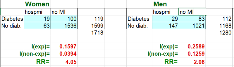
Magnitude of confounding = (crude RR- adjusted RR) / (adjusted RR) = (2.74-2.56) / 2.56 = 0.07 =7%. Since this is less than 10%, there was little evidence of confounding. However, the risk ratio in females was nearly twice that in males, so there was evidence of possible effect measure modification.'
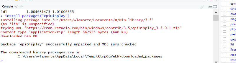
You can do a stratified analysis of a case-control study using another imported package call "epiDisplay", but the package has to be installed once, and then it has to be loaded each time you want to use it.
To install it, go to the lower right windon in R Studio and click on the "install" tab.

Another window opens. Enter "epiDisplay" as shown below.
Click on "Install at the bottom of the window. The package should be installed, and you should see the following text appear in the Console window.
The installation procedure above only needs to be done once, but you need to load the package each time you use it by including the following line of code in your script:
library(epiDisplay)
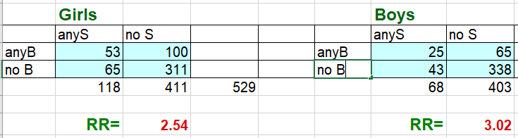
> # Stratified with epiDisplay
> library(epiDisplay)
> mhor(anyB,anyS,female)
Stratified analysis by female
OR lower lim. upper lim. P value
female 0 3.01 1.64 5.46 1.86e-04
female 1 2.53 1.61 3.97 2.84e-05
M-H combined 2.69 1.92 3.79 5.02e-09
M-H Chi2(1) = 34.18 , P value = 0
Homogeneity test, chi-squared 1 d.f. = 0.24 , P value = 0.627
Interpretation: The crude odds ratio for the assocation between anyB and anyS was 2.84. After adjusting for confounding by sex, the Mantel-Haenszel odds ratio was 2.69 (p<0.0001). The magnitude of confounding was (crude OR- adjusted OR) / adjusted OR = (2.84-2.69) / 2.69 = 0.056 = 5.6%. THis is less than a 10% difference, so there was little or no confounding by sex.
When looking for a potential association between two continuously distributed measurement variables, we can begin by creating a scatter plot to determine whether there is a reasonably linear relationship between them. The possible values of the exposure variable (i.e., predictor or independent variable) are shown on the horizontal axis (the X-axis), and possible values of the outcome (the dependent variable) are shown on the vertical axis (the Y-axis).
plot(Savings~Week)
You can add the regression line to the scatter plot with the abline() function.
abline(lm(Savings~Week))
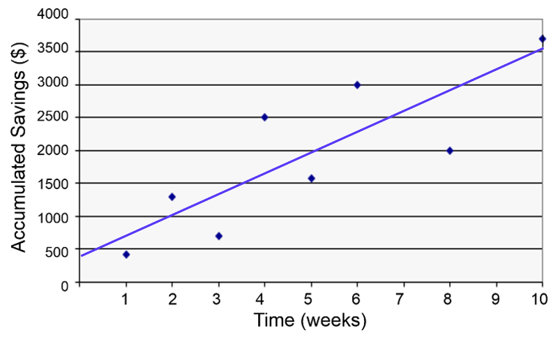
The regression line is determined from a mathematic model that minimizes the distance between the observation points and the line. The correlation coefficient (r) indicates how closely the individual observation points conform to the regression line.
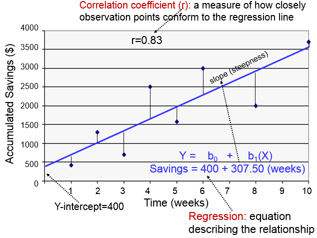
The steepness of the line is the slope, which is a measure of how many units the Y-variable changes for each increment in the X-variable; in this case the slope provides an estimate of the average weekly increase in savings. Finally, the Y-intercept is the value of Y when the X value is 0; one can think of this as a starting or basal value, but it is not always relevant. In this case, the Y-intercept is $400 suggesting that this individual had that much in savings at the beginning, but this may not be the case. She may have had nothing, but saved a little less than $500 after one week.
Notice also that with this kind of analysis the relationship between two measurement variables can be summarized with a simple linear regression equation, the general form of which is:

where b0 is the value of the Y-intercept and b1 is the slope or coefficient. From this model one can make predictions about accumulated savings at a particular point in time by specifying the time (X) that has elapsed. In this example, the equation describing the regression is:
SAVINGS=400 + 307.50 (weeks)
cor(xvar, yvar)
This calculates the correlation coefficient for two continuously distributed variables. You should not use this for categorical or dichotomous variables.
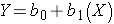
cor(hgt_inch,weight)
[1] 0.5767638
cor.test(xvar, yvar)
This calculates the correlation coefficient and 95% confidence interval of the correlation coefficient and calculates the p-value for the alternative hypothesis that the correlation coefficient is not equal to 0.
cor.test(hgt_inch,weight)
Pearson's product-moment correlation
data: hgt_inch and weightt = 40.374, df = 3270, p-value < 2.2e-16
alternative hypothesis: true correlation is not equal to 095 percent confidence interval:
0.5534352 0.5991882sample estimates:
****cor
0.5767638
reg_output_name<-lm(yvar~xvar)
summary(reg_output_name)
Linear regression in R is a two part command. The first command fits a linear regression line with yvar (outcome) and xvar (predictor) to the "reg_output_name" (you can use any name). The summary() command prints out the regression equation and summary statistics. Be sure to use the ~ character between the Y-variable (outcome) and the X-variable (predictor). Here is a simple linear regression of weight as a function of height from the Weymouth Health Survey.
plot(weight~hgt_inch)
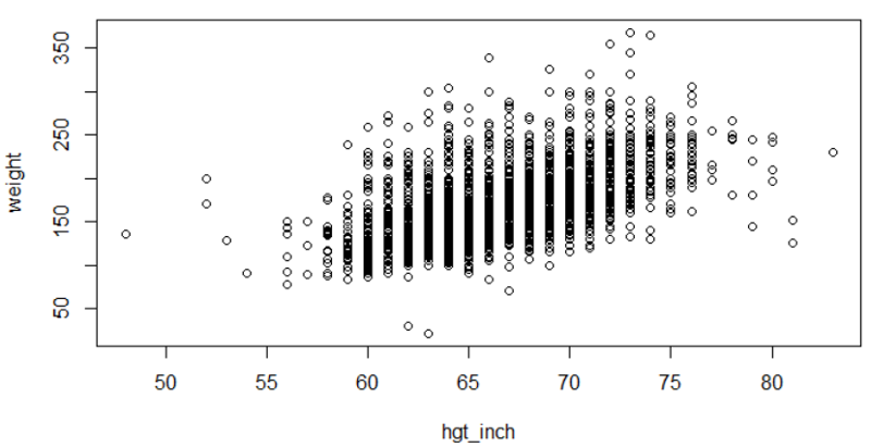
myreg<-lm(weight~hgt_inch)
abline(myreg, col = 'red')
summary(myreg)
Call:
lm(formula = weight ~ hgt_inch)
Residuals:
*****Min *****1Q Median ****3Q ****Max
-127.413 -21.824 -4.837 15.897 172.451
Coefficients:
*************Estimate Std. Error t value Pr(>|t|)
(Intercept) -211.4321 ****9.4202 *-22.45 *<2e-16 ***
hgt_inch *******5.7118 ****0.141 ***40.37 *<2e-16 ***
---
Signif. codes: 0 '***' 0.001 '**' 0.01 '*' 0.05 '.' 0.1 ' ' 1
Residual standard error: 32.64 on 3270 degrees of freedom
Multiple R-squared: 0.3327, Adjusted R-squared: 0.3325
F-statistic: 1630 on 1 and 3270 DF, p-value: < 2.2e-16
In the example below I am using part of the data from the Framingham Heart Study to determine whether body mass index (bmi) is associated with systolic blood pressure (sysbp).
First, I run a simple linear regression to assess the crude (unadjusted) association between bmi and sysbp.
# Simple Linear Regression
> summary(lm(sysbp~bmi))
Call:
lm(formula = sysbp ~ bmi)
Residuals:
Min 1Q Median 3Q Max
-49.960 -15.973 -2.991 13.389 116.933
Coefficients:
Estimate Std. Error t value Pr(>|t|)
(Intercept) 108.9627 2.6391 41.29 <2e-16 ***
bmi 1.1959 0.1008 11.87 <2e-16 ***
---
Signif. codes: 0 '***' 0.001 '**' 0.01 '*' 0.05 '.' 0.1 ' ' 1
Residual standard error: 22.12 on 2996 degrees of freedom
Multiple R-squared: 0.04489, Adjusted R-squared: 0.04457
F-statistic: 140.8 on 1 and 2996 DF, p-value: < 2.2e-16
Interpretation: BMI is significant related to systolic blood pressure (p<0.0001). Each increment in BMI is associated with an increase in sysbp of 1.2 mm Hg.
> #Multiple linear Regression
> summary(lm(sysbp~bmi + age + male + ldl + hdl +cursmoke))
Call:
lm(formula = sysbp ~ bmi + age + male + ldl + hdl + cursmoke)
Residuals:
Min 1Q Median 3Q Max
-54.981 -14.886 -2.319 11.703 105.840
Coefficients:
Estimate Std. Error t value Pr(>|t|)
(Intercept) 45.885480 4.723993 9.713 <2e-16 ***
bmi *1.263627 0.097482 *12.963 <2e-16 ***
age 0.925972 0.047140 *19.643 <2e-16 ***
male -0.896683 0.818306 *-1.096 0.273
ldl 0.021030 0.008265 2.545 *0.011 *
hdl 0.041834 0.026281 1.592 *0.112
cursmoke -0.499081 0.836412 **-0.597 *0.551
---
Signif. codes: 0 '***' 0.001 '**' 0.01 '*' 0.05 '.' 0.1 ' ' 1
Residual standard error: 20.68 on 2991 degrees of freedom
Multiple R-squared: 0.166, Adjusted R-squared: 0.1643
F-statistic: 99.22 on 6 and 2991 DF, p-value: < 2.2e-16
Interpetation: After adjusting for age, sex, LDL, HDL, and current smoking, BMI was still significantly associated with systolic blood pressure. Each unit increase in BMI was associated with a modest increase in systolic blood pressure of about 1.3 mm Hg on average (p<0.0001). The adjusted estimate for BMI was similar to the crude estimate.
I am again using the Framinghams data set, but now my goal is to test whether there is an association between diabetes and odds of being hospitalized for a myocardial infarction (hospmi). I begin by looking at the crude association. So, now the outcome of interest (hospmi) is a dichotomous variable, and I have to use logistic regression instead of linear regression.
# First I will examine the crude association with a simple chi-squared test
> table(diabetes,hospmi)
hospmi
diabetes 0 1
0 **2557 210
1 *183 48
> library(epitools)
> oddsratio.wald(table(diabetes,hospmi))
$data
hospmi
diabetes 0 1 Total
***0 2557 210 2767
***1 183 48 231
*Total **2740 *258 2998
$measure
odds ratio with 95% C.I.
diabetes estimate lower upper
0 1.000000 NA **NA
1 3.193755 2.256038 4.521233
$p.value
two-sided
diabetes midp.exact fisher.exact chi.square
0 NA NA NA
1 1.945462e-09 1.88176e-09 6.548224e-12
$correction
[1] FALSE
attr(,"method")
[1] "Unconditional MLE & normal approximation (Wald) CI"
Interpretation: Subjects with diabetes had 1.95 times the odds of being hospitalized for a myocardial infarction compared to subjects without diabetes (p<0.0001)
# Multiple Logistic Regression
> log.out <-glm(hospmi~diabetes + age + male + bmi + sysbp + diabp + hdl + ldl,
+ family=binomial (link=logit))
> summary(log.out)
Call:
glm(formula = hospmi ~ diabetes + age + male + bmi + sysbp +
diabp + hdl + ldl, family = binomial(link = logit))
Deviance Residuals:
Min 1Q Median *3Q *Max
-1.3615 -0.4634 -0.3282 -0.2277 2.7531
Coefficients:
Estimate Std. Error z value Pr(>|z|)
(Intercept) -5.946249 0.961247 -6.186 6.17e-10 ***
diabetes 0.946976 0.192002 4.932 8.13e-07 ***
age 0.016407 0.009186 1.786 0.074088 .
male 1.197212 0.153976 7.775 7.52e-15 ***
bmi -0.003890 0.018470 -0.211 0.833172
sysbp 0.012896 0.004114 3.135 0.001721 **
diabp -0.005405 0.007965 -0.679 0.497354
hdl -0.017798 0.005306 -3.354 0.000795 ***
ldl 0.007328 0.001374 *5.334 9.62e-08 ***
---
Signif. codes: 0 '***' 0.001 '**' 0.01 '*' 0.05 '.' 0.1 ' ' 1
(Dispersion parameter for binomial family taken to be 1)
Null deviance: 1758.7 on 2997 degrees of freedom
Residual deviance: 1579.5 on 2989 degrees of freedom
AIC: 1597.5
Number of Fisher Scoring iterations: 6
# The next command asks R to provide the adjusted odds ratios for each variable in the model
> exp(log.out$coeff)
(Intercept) diabetes age male **bmi sysbp diabp
0.002615633 2.577901246 1.016542819 3.310874851 0.996117094 1.012979017 0.994609173
**hdl ldl
0.982359551 1.007354740
# The next command asks for the 95% confidence intervals for the adjusted odds ratios.
> exp(confint(log.out))
Waiting for profiling to be done...
2.5 % 97.5 %
(Intercept) 0.000392781 0.01703735
diabetes 1.755767291 3.73167495
age 0.998370449 1.03500180
male 2.457227924 4.49622942
bmi 0.960202678 1.03233392
sysbp 1.004774973 1.02112476
diabp 0.979236759 1.01032182
hdl 0.972038277 0.99246563
ldl 1.004631473 1.01006555
Interpretation: After adjusting for age, sex, BMI systolic and diastolic blood pressure, HDL cholesterol, and LDL cholesterol, diabetics had 0.95 times the odds of being hospitalized for a myocardial infarction compared to non-diabetics. Since the crude odds ratio was 1.95, this indicates that the association between diabetes and hospitalizaiton for MI was confounded by one or more of these other risk factors.
Plots have lots of options for labeling. To use the plot options, you add them to the basic plot command separated by commas. Here are some common plot options.
main="Main Title"
ylab = "Y-axis label"
xlab="X-axis label "
ylim = c(lower, upper)
xlim = c(lower, upper)
names=c("label1", "label2" [,... "labelx"])
hist(varname)
Creates a histogram for a continuously distributed variable.
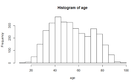
hist(age, main = "Age Distribution of Weymouth Adults", xlab = "Age")
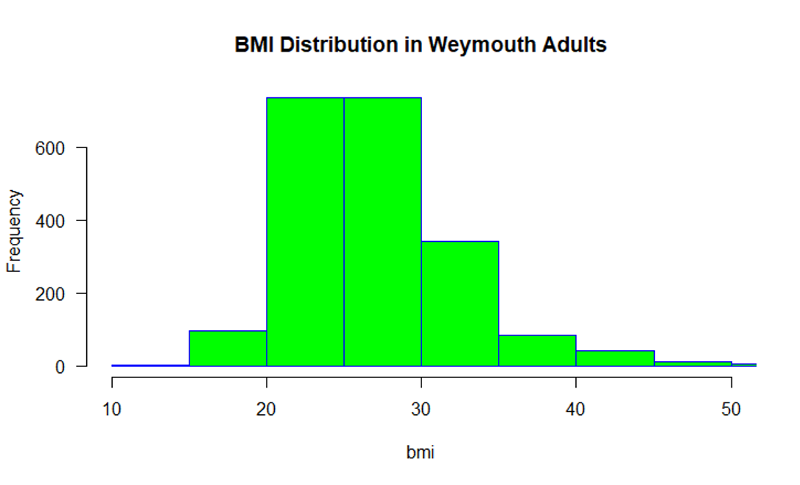
hist (bmi, main="BMI Distribution in Weymouth Adults",
xlab = "BMI", border="blue", col="green", xlim=c(10,50,
las=1, breaks=8)
boxplot(varname)
Creates a boxplot for a continuously distributed variable.
The code below gives it a title and a label for the Y-axis
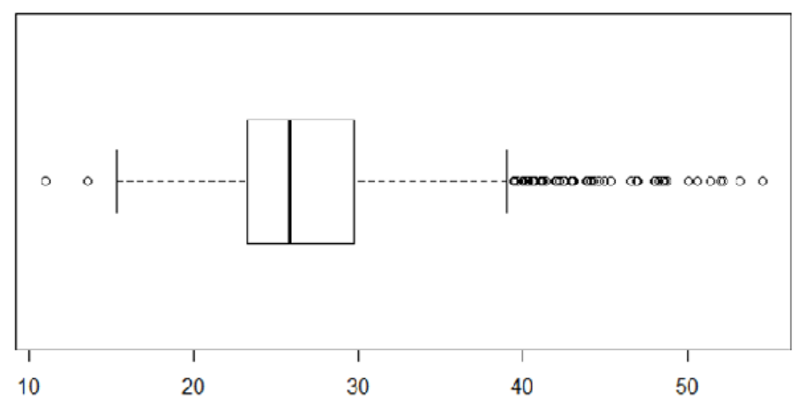
boxplot (bmi, main = "BMI Distribution in Weymouth Adults", ylab = "BMI")
boxplot(bmi, horizontal = TRUE)
boxplot(varname~groupname)
Creates a boxplot of varname for each groupname.
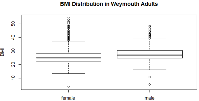
boxplot(bmi~gender, main="BMI Distribution in Weymouth Adults", ylab = "BMI")
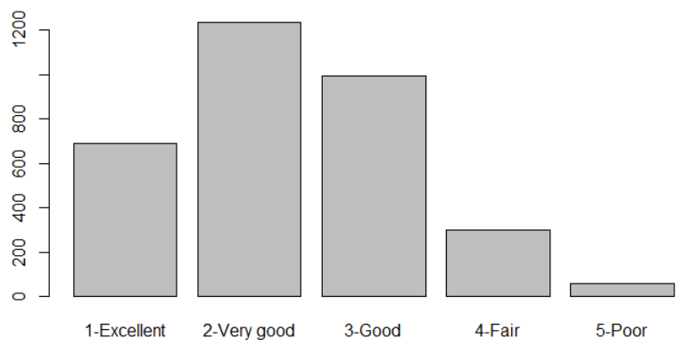
barplot(table(varname))
Creates a barplot of frequencies by varname
table(gen_health)
barplot(table(gen_health))
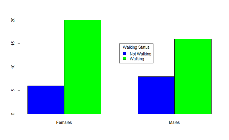
Example: Producing grouped bar charts for whether an infant could walk by 1 year of age (outcome) stratified by sex (exposure).
"Sexmale" was coded as "1" for males and "0" for females. The dichotomous outcome, "By1year", is an indicator variable, where "1" indicated that the infant could walk by 1 year and "0" indicated that the infant could not walk by 1 year.
> barplot(table(By1year,Sexmale),beside=TRUE,
names=c("Females","Males"),col=c("blue","green"))
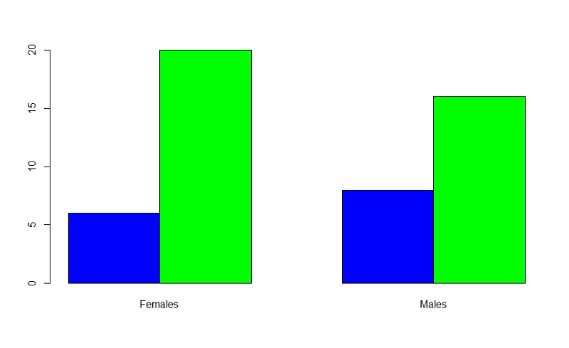
In the table statement, the first variable is the outcome plotted on the y axis, the exposure is the second variable. If you want to add a legend, you could use the following code:
> barplot(table(By1year,Sexmale),beside=TRUE,
names=c("Females","Males"),col=c("blue","green"))
> legend(x=3.5,y=15,legend=c("Not Walking","Walking"),fill=c("blue","green"),
title="Walking Status")
Bar plots should ideally just show the proportion of individual who have a dichotomous outcome. There is no need to also show the proportion who do not have it. This can be accomplished using the matrix command to create an abbreviated table.
This can be accomplished using the matrix command to create an abbreviated table. The example below uses data from the Framingham Heart Study to create a bar plot comparing the incidence of myocardial infarction or fatal coronary heart disease (mifchd) in diabetics and non-diabetics. We first use the table() and prop.table() commands to get the proportions.
> table(diabetes,mifchd)
mifchd
diabetes 0 1
0 2452 316
1 162 69
> prop.table(table(diabetes,mifchd),1)
mifchd
diabetes 0 1
0 0.8858382 0.1141618
1 0.7012987 0.2987013
The only relevant information is the proportion with the outcome in each exposure group in the second column of the prop.table. Therefore, we create an abbreviated table using the matrix command and placing the incidence in diabetics first.
> mybar<-matrix(c(0.2987,0.1146))
Now we can create the bar plot:
> barplot(mybar, beside=TRUE,ylim = c(0,1), names=c("Diabetics", "Non-diabetics"), ylab="Incidence of MI or FCHD",main = "Incidence of MI or FCHD in Diabetics & Non-diabetics")
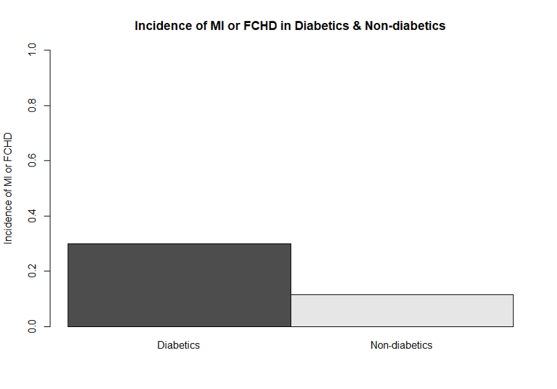
This bar plot is easier to understand without the extraneous bars showing the proportion who did not develop the outcome. Journals generally do not want colored graphs unless it is absolutely necessary. By omitting color designations, the default settings resulted in a black and a gray bar.
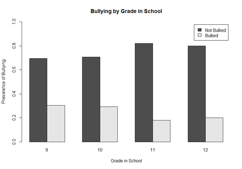
This next example is based on data from the Youth Risk Behavior Surveillance System, a cross-section survey conducted periodically by the Center for Disease Control. This survey asked high school students about whether they had been bullied in school or online and whether they had contemplated or attempted suicide. The graph below illustrates the prevalence of any bullying (anyB) by grade in high school.
First, we get the counts of bullying by grade and then use prop.table() to get the proportions (prevalence).
> table(anyB,grade)
grade
anyB 9 10 11 12
0 169 176 225 187
1 74 73 49 47
> prop.table(table(anyB,grade),2)
grade
anyB 9 10 11 12
0 0.6954733 0.7068273 0.8211679 0.7991453
1 0.3045267 0.2931727 0.1788321 0.2008547
Next we create the bar plot with a legend. The range of the Y-axis has been set to 0 to 1, and we have also provided labels for the X- and Y-axes, a legend, and a main title.
> barplot(gradetable,beside=TRUE, xlab= "Grade in School", ylab= "Prevalence of Bullying", ylim = c(0,1),legend=c("Not Bullied","Bullied"), main="Bullying by Grade in School" )
This illustrates the use of a legend, but, again, the graph would be improved by eliminating the bars that show the prevalence of NOT being bullied. We can once again achieve that by using the matrix command to create a table with only the proportions of those who were bullied as shown below.
> gradetable2<-matrix(c(0.304,0.293,0.17,0.20))
> barplot(gradetable2,beside=TRUE, names=c(9,10,11,12),xlab= "Grade in School", ylab= "Prevalence of Bullying", ylim = c(0,1), main="Bullying by Grade in School")
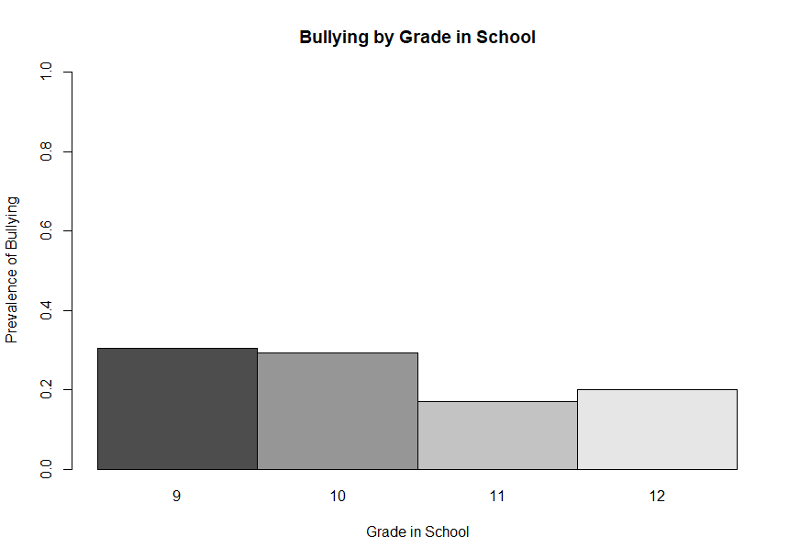
This simpler bar plot more clearly shows that bullying is more prevalent in grades 9 and 10 than it is in the upperclassmen.
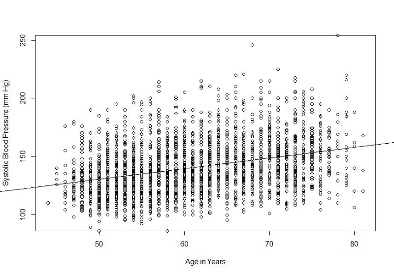
plot(yvar~xvar)
Creates a plot with a point for each observation for xvar and yvar.
plot(sysbp~age)
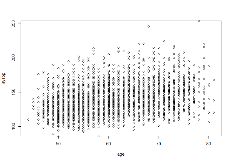
This would be more informative if we ran a simple linear regression and added the "abline()" command after the line of code creating the plot. We should also add more explicit labels for the X- and Y-axes. These improvements are shown below.
> myreg<-lm(sysbp~age)
> plot(sysbp~age, xlab= "Age in Years", ylab="Systolic Blood Pressure (mm Hg)")
> abline(myreg)