


T-Tests
One Sample t-test
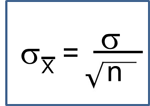
This is used when a single sample is compared to a "usual" or historic population mean.
t.test(varname, μ =population mean)
Example: The mean IQ in the population=100. Do children who were born prematurely have lower IQ? Investigators measured the IQ of n=100 children who had been born prematurely. The mean IQ in this sample was 95.8 with a standard deviation (SD) of 17.5. What is the probability that a sample of 100 will have a mean IQ of 95.8 (or less)?

pt(-2.4,99)
[1] 0.009132283
However, this can be done completely with R if you have the raw data set.
t.test(iq,mu=100)
One Sample t-test
data: iq
t = -2.3801, df = 99, p-value = 0.01922
alternative hypothesis: true mean is not equal to 100
95 percent confidence interval:
92.35365 99.30635
sample estimates:
mean of x
95.83
One-Tailed and Two-Tailed T-Tests
In most cases, it is appropriate to do a two-tailed test for which the alternative hypothesis is that there is a difference without specifying which group is expected to be greater. However, there are situations for which a one-tailed test is accepable. If no option is specified, R will automatically perform the more conservative two-tailed comparison, but you can specify a one-tailed test.
In the example below, we test the null hypothesis that the bonedensity in a sample of people is not equal to one. In the first comparison, we do not specify whether to do a one-tailed or two-tailed test, so R automatically performs a two-tailed test.
t.test(bonedensity,mu=1)
One Sample t-test
data: bonedensity
t = 1.2205, df = 34, p-value = 0.2307
alternative hypothesis: true mean is not equal to 1
95 percent confidence interval:
0.9790988 1.0837583
sample estimates:
mean of x
1.031429
The difference was not statistically significant (p=0.23).
Next, the test is repeated as a one-tailed test specifying that we expect the sample to have a mean bonedensity greater than 1.
t.test(bonedensity,mu=1, alternative="greater")
One Sample t-test
data: bonedensity
t = 1.2205, df = 34, p-value = 0.1153
alternative hypothesis: true mean is greater than 1
95 percent confidence interval:
0.9878877 Inf
sample estimates:
mean of x
1.031429
The difference is once again not statistically significant (p=0.1153), but note that the p-value is half of that obtained with the more conservative two-tailed test.
If your alternative hypothesis is that the mean bonedensity for the sample is less than 1, you would use the following code:
t.test(bonedensity,mu=1, alternative="less")
T-test to Compare Two Independent Sample Means (unpaired t-test)
This is used to compare means between two independent samples. This test would be appropriate if you were comparing means in two different groups of people in a clinical trial when the two groups were randomly allocated to receive different treatments.
There are two options for this test - one when the variances of the two groups are approximately equal and another when they are not. The variance is the square of the standard deviation.
To determine whether the variances for the two samples are reasonably similar, compute the ratio of the sample variances.
- If the ratio is between 0.5-2.0, the equal variance assumption is met, and you can use the var.equal=TRUE option.
t.test(varname ~ groupname, var.equal=TRUE)
- If the ratio of the sample variances is less than 0.5 or greater than 2.0, use the var.equal=FALSE option.
t.test(varname ~ groupname, var.equal=FALSE)
Example: I want to compare mean bonedensity measures in subjects who exercise regularly and those who do not.
# First I use tapply() to get the two standard deviations
tapply(bonedensity,exercise,sd)
0 1
0.1571489 0.1275296
# Then I find the ratio of the squared standard deviations
0.157^2/0.1286^2
[1] 1.49045
# The ratio is between 0.5 and 2.0, so I can use the equal variance option
# If you do not specify the var.equal option, it will assume they are unequal
t.test(bonedensity~exercise,var.equal=TRUE)
Two Sample t-test
data: bonedensity by exercise
t = -2.0885, df = 33, p-value = 0.04455
alternative hypothesis: true difference in means is not equal to 0
95 percent confidence interval:
-0.204653969 -0.002679364
sample estimates:
mean in group 0 mean in group 1
0.987000 1.090667
IMPORTANT NOTE!
When performing a t-test for independent groups, be sure to separate the variables with the ~ character. Do not separate them with a comma.
Below is en ecample of the correct way and the incorrect way using the same data set.
Correct Way:
> t.test(height~anyS,var.equal = TRUE)
Two Sample t-test
data: height by anyS t = 3.3696, df = 998, p-value = 0.0007816
alternative hypothesis: true difference in means is not equal to 0 95 percent confidence interval:
0.01217630 0.04613444
sample estimates:
mean in group 0 mean in group 1
1.694263 1.665108
Incorrect Way:
> t.test(height,anyS,var.equal = TRUE)
Two Sample t-test
data: height and anyS t = 117.71, df = 1998, p-value < 2.2e-16
alternative hypothesis: true difference in means is not equal to 0 95 percent confidence interval:
1.477801 1.527879
sample estimates:
mean of x mean of y 1.68884 0.18600
Note that the second method is comparing the mean height to the mean value of the dichotomous group variable, which makes no sense. It is giving an incorrect t-statistic, incorrect degrees of freedom, and an incorrect p-value.
t-Test for Comparing Two Matched or Paired Samples (paired t-test)
t.test(varname1, varname2,paired=TRUE)
This is used for comparing the means of paired or matched samples, such as the following:
- A sample of subjects take a test to gauge their knowledge of HIV transmission risk. They are then given a training on HIV transmission. Six weeks later all subjects are again tested on their knowledge of HIV transmission. For each individual the post-training score is subjtracted from the pre-training score, and the mean difference in pre and post scores in computed.
- A sample of identical twins who were separated at birth is identified, and their IQa are measured an compared using a t-test for matched samples.
Example: Early in the HIV epidemic, there was poor knowledge of HIV transmission risks among health care staff. A training was developed to improve knowledge and attitudes around HIV disease. All subjects were given a test to assess their knowledge before the training and again several weeks after the training. The table below shows their scores before (Kscore1) and after the training (Kscore2).
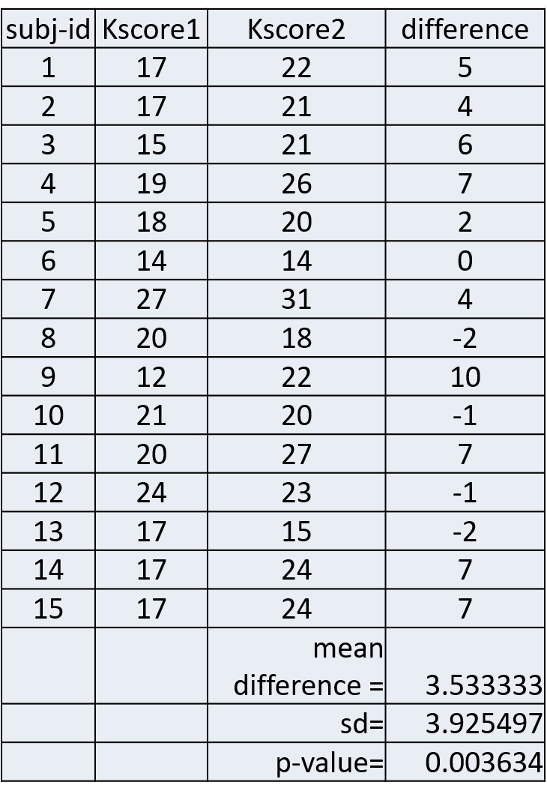
The column on the far right shows the difference in score for each subject and the mean differenence was 3.53333. The null hypothesis is that the mean difference is 0. Is there sufficient evidence to reject the null hypothesis and accept the alternative hypothesis that the before and after scores differed significantly?
This was tested using R as shown below.
# First the means scores before and after the test were calculated
mean(Kscore1)
[1] 18.33333
mean(Kscore2)
[1] 21.86667
# Then a paired t-test was performed
t.test(Kscore2,Kscore1,paired=TRUE)
Paired t-test
data: Kscore2 and Kscore1
t = 3.4861, df = 14, p-value = 0.003634
alternative hypothesis: true difference in means is not equal to 0
95 percent confidence interval:
1.359466 5.707201
sample estimates:
mean of the differences
3.533333
Interpretation: The mean difference was 3.533333. The confidence interval for the mean difference is from 1.36 to 5.71. We can conclude that on average, test scores improved 3.5 points after the training. With 95% confidence, the true mean improvement in scores was between 1.36 and 5.71 points.