


Risk Ratios and Odds Ratios with 95% Confidence Interval
riskratio.wald(exposure_var, outcome_var)
When dealing with a cohort study or a clinical trial, this command calculates a risk ratio and 95% confidence interval for the risk ratio and also performs a chi-squared test.
oddsatio.wald(exposure_var, outcome_var)
When dealing with a case-control study, this command calculates an odds ratio and 95% confidence interval for the odds ratio and also performs a chi-squared test.
Note: The "base package" in R does not have this function, but R has supplemental packages that can be loaded to add additional analytical tools, including confidence intervals for RR and OR. These tools are in the "epitools" package. You need to install the Epitools package into your version of R once from the Console in R Studio. Then, whenever you want to use the "wald" functions, you need to include a line in your script that will load the package.
Installing the Epitools Package
Go to the Console window (lower left) in R and type:
>install.packages("epitools")
Be sure to include the quotation marks around "epitools". R wil install the package and display the following:
Installing package into 'C:/Users/wlamorte/Documents/R/win-library/3.5' (as 'lib' is unspecified) trying URL 'https://cran.rstudio.com/bin/windows/contrib/3.5/epitools_0.5-10.1.zip' Content type 'application/zip' length 317397 bytes (309 KB)
Loading the Epitools Package When You Want to Use It
You only have to install the epitools package once, but you have to load it up each time you use it by including the following line of code in your script before the riskratio.wald command.
library(epitools)
R responds with:
Warning message: package 'epitools' was built under R version 3.4.2
Computing a Risk Ratio and 95% Confidence Limits from a Data Set
I have a data set from the Framingham Heart Study, and I want to compute the risk ratio for the association between type 2 diabetes ("diabetes") and risk of being hospitalized with a myocardial infarction ("hospmi"). I begin by creating a contingency table with the table() command.
table(diabetes,hospmi)
************hospmi
diabetes 0 1
*******0 2557 210
*******1 183 48
Then, to compute the risk ratio and confidence limits, I insert the table parameters into the riskratio.wald() function:
riskratio.wald(table(diabetes,hospmi))
$data
**************hospmi
diabetes ***0 1 Total
*******0 2557 210 2767
*******1 183 48 231
Total ***2740 258 2998
$measure
risk ratio with 95% C.I.
diabetes estimate lower upper
*******0 1.00000 NA NA
*******1 *2.73791 2.062282 3.63488
NOTE: I changed the text color to red to call it to your attention. R does not do this.
Using the same data for illustration, I can similarly compute an odds ratio and its confidence interval using the oddsratio.wald() function:
oddsratio.wald(table(diabetes,hospmi))
$data
hospmi
diabetes **0 1 Total
*******0 2557 210 2767
*******1 183 48 231
***Total ***2740 258 2998
$measure
odds ratio with 95% C.I.
diabetes estimate lower upper
*******0 1.000000 NA NA
*******1 *3.193755 2.256038 4.521233
Computing Risk Ratios and Odds Ratios using the epiR package
There are many extra packages for R and many alternate ways to compute things. Another package that is useful for risk ratios and odds ratios is the epiR package. Like the epi.tools package, it must be installed once, and then it must be loaded into each script in which it is used.
To do the one time installation, go to the lower right window and click on the Packages tab and then on the Install tab. In the window that opens, enter epiR as shown below.
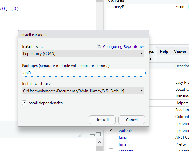
Then click on the Install button, and wait a few seconds while the package is installed.
Then, to use the program, you must load it into your script. Here is an example of its use in calculating a risk ratio, the 95% confidence interval for the risk ratio, the risk difference, and the attributable fraction.
In the example below, I use a data set from the Framingham Heart Study to create a table called "TAB" that summarizes the occurrence of being hospitalized for a myocardial infarction (hospmi) for diabetics and non-diabetics. I then print TAB to verify the counts, then call up the epiR package, and then give the command
> epi.2by2(TAB,method="cohort.count", conf.level = 0.95)
This asks R to use the data object called "TAB" and to analyze it as counts in a cohort study and compute the 95% confidence interval for the risk ratio.
> TAB<-table(diabetes, hospmi)
> TAB
hospmi
diabetes 0 1
0 2557 210
1 183 48
> library(epiR)
Package epiR 1.0-15 is loaded
Type help(epi.about) for summary information
Type browseVignettes(package = 'epiR') to learn how to use epiR for applied epidemiological analyses
> epi.2by2(TAB,method="cohort.count", conf.level = 0.95)
Outcome + Outcome - Total Inc risk * Odds
Exposed + 2557 210 2767 92.4 12.18
Exposed - 183 48 231 79.2 3.81
Total 2740 258 2998 91.4 10.62
Point estimates and 95% CIs:
-------------------------------------------------------------------
Inc risk ratio 1.17 (1.09, 1.25)
Odds ratio 3.19 (2.26, 4.52)
Attrib risk * 13.19 (7.87, 18.51)
Attrib risk in population * 12.17 (6.85, 17.50)
Attrib fraction in exposed (%) 14.27 (8.34, 19.82)
Attrib fraction in population (%) 13.32 (7.73, 18.57)
-------------------------------------------------------------------
Test that OR = 1: chi2(1) = 47.158 Pr>chi2 = <0.001
Wald confidence limits
CI: confidence interval
* Outcomes per 100 population units
NOTE: The "Attributable Risk (Attrib risk;) is the risk difference. The last two measures can be ignored for PH717. Also, since the Framingham Heart Study was a cohort study, we can ignore the odds ratio.
epi R for Case-Control Studies
If we were analyzying a table from a case control study, we would use the following command:
> epi.2by2(TAB, method="case.control", conf.level = 0.95)
Outcome + Outcome - Total Prevalence * Odds
Exposed + 2557 210 2767 92.4 12.18
Exposed - 183 48 231 79.2 3.81
Total 2740 258 2998 91.4 10.62
Point estimates and 95% CIs:
-------------------------------------------------------------------
Odds ratio (W) 3.19 (2.26, 4.52)
Attrib prevalence * 13.19 (7.87, 18.51)
Attrib prevalence in population * 12.17 (6.85, 17.50)
Attrib fraction (est) in exposed (%) 68.67 (54.64, 78.07)
Attrib fraction (est) in population (%) 64.10 (51.97, 73.17)
-------------------------------------------------------------------
Test that OR = 1: chi2(1) = 47.158 Pr>chi2 = <0.001
Wald confidence limits
CI: confidence interval
* Outcomes per 100 population units
Here we are only interested in the odds ratio and its 95% confidence interval. The other output can be ignored.
Computing a Risk Ratio and 95% Confidence Limits When you DON'T Have a Data Set
The preceding illustration showed how you use a table() command to create a contingency table that can be interpreted by riskratio.wald() or oddsratio.wald from a data set. However, suppose you don't have the raw data set, and you just have the counts in a contingency table. In this situation, the first task is to create a contingency table that R can interpret correctly in order to compute RR or OR and the corresponding 95% confidence interval.
Creating a contingency table that R can understand
When R executes the table() command, it does so with the lowest named variables first in both the rows and columns. Here is the table showing the distribution of being hospitalized for a myocardial infarction (hospmi) among those with and without type 2 diabetes.
**************hospmi
diabetes ***0 1 Total
*******0 2557 210 2767
*******1 *183 48 231
Total **2740 258 2998
Note that it lists those without diabetes in the first row, and it list those without having been hospitalized for MI in the first column, since 0 comes before 1.
Important: Adhering to this "lowest first" format will become important if you want to run riskratio.wald() if you don't have a raw data. If you are given the counts in a contingency table without access to the raw data set you will need to create a contingency table in R that adheres to this structure using the matrix() function, as explained below.
Note also that "riskratio.wald" can be used to analyze prevalence data also. In this case, the procedure calculates a prevalence ratio and its 95% confidence limits.
If you are given the counts in a contingency table, i.e., you do not have the raw data set, you can re-create the table in R and then compute the risk ratio and its 95% confidence limits using the riskratio.wald() function in Epitools.
| No CVD (0) | CVD (1) | Total | |
|---|---|---|---|
| No HTN (0) | **********1017 | **********165 | ********1182 |
| HTN (1) | **********2260 | **********992 | ********3252 |
This is where the orientation of the contingency table is critical, i.e., with the unexposed (reference) group in the first row and the subjects without the outcome in the first column.
The contingency table for R is created using the matrix function, entering the data for the first column, then second column as follows:
R Code:
# the 1st line below creates the contingency table; the 2nd line prints the table so you can check the orientation of the numbers
RRtable<-matrix(c(1017,2260,165,992),nrow = 2, ncol = 2)
RRtable
[,1] [,2]
[1,] 1017 165
[2,] 2260 992
# The next line asks R to compute the RR and 95% confidence interval
riskratio.wald(RRtable)
$data
*******Outcome
Predictor Disease1 Disease2 Total
Exposed1 1017 165 1182
Exposed2 2260 992 3252
Total 3277 1157 4434
$measure
risk ratio with 95% C.I.
Predictor estimate *lower upper
Exposed1 **1.000000 NA *****NA
Exposed2 ****2.185217 *1.879441 2.540742
NOTE: The "Exposed2 line shows the risk ratio and the lower and upper limits of its 95% confidence interval. I changed the text color to red to bring this to your attention. R does not show this in red.
$p.value
two-sided
Predictor midp.exact fisher.exact chi.square
Exposed1 NA ******NA**********NA
Exposed2 0 *7.357611e-31 *1.35953e-28zz
NOTE: The last entry in the line above shows the p-value from the chi-squared test, which I highlighted in red. R does not show this in red.
$correction [1] FALSE
attr(,"method") [1] "Unconditional MLE & normal approlimation (Wald) CI"
The risk ratio and 95% confidence interval are listed in the output under $measure.
An Alternative Method for Reading Table Data into Riskratio.wald
The table below summarizes the prevalence of migraine headaches in people exposed to low or high concentrations of flame retardants. The table is already oriented showing the least exposed in the first column and the non-diseased subjects in the first column, i.e., the format required by RStudio.
|
|
Disease - |
Disease + |
Total |
|---|---|---|---|
|
Exp. - |
380 |
20 |
400 |
|
Exp. + |
540 |
60 |
600 |
After loading epitools, I can employ riskratio.wald to compute the prevalence ratio using the previously described method to create a table object called "mytab" and using the matrix command to read the data by COLUMNS and specifying the numbers of rows and columns.
mytab<-matrix(c(380,540,20,60),nrow=2,ncol=2)
riskratio.wald(mytab)
An alternative method is to have R read the count by ROWS using the following command:
riskratio.wald(c(380,20,540,60))
Note that this method does not use the matrix function, and it does not require one to specify the number of rows and columns. Nevertheless, both methods give identical output.
$data
Outcome
Predictor Disease1 Disease2 Total
Exposed1 380 20 400
Exposed2 540 60 600
Total 920 80 1000
$measure
risk ratio with 95% C.I.
Predictor estimate lower upper
Exposed1 1 NA NA
Exposed2 2 1.225264 3.264603
$p.value
two-sided
Predictor midp.exact fisher.exact chi.square
Exposed1 NA NA NA
Exposed2 0.003676476 0.004173438 0.004300957
Computing an Odds and 95% Confidence Limits When you DON'T Have a Data Set
This procedure is similar to the preceding section, except that you will use the oddsratio.wald() function. Once again, it is critical that you use the matrix command correctly in order to create a contingency table that will give the correct results. We will illustrate using the same counts as in the example above.
| No CVD (0) | CVD (1) | Total | |
|---|---|---|---|
| No HTN (0) | **********1017 | **********165 | ********1182 |
| HTN (1) | **********2260 | **********992 | ********3252 |
ORtable<-matrix(c(1017,2260,165,992),nrow = 2, ncol = 2)
ORtable
[,1] [,2]
[1,] 1017 165
[2,] 2260 992
oddsratio.wald(ORtable)
$data
Outcome
Predictor Disease1 Disease2 Total
Exposed1 1017 165 1182
Exposed2 2260 992 3252
Total 3277 1157 4434
$measure
odds ratio with 95% C.I.
Predictor estimate lower upper
Exposed1 *1.000000 NA ****NA
Exposed2 **2.705455 *2.258339 *3.241093
$p.value two-sided
Predictor midp.exact fisher.exact chi.square
Exposed1 NA *********NA**********NA
Exposed2 0 *7.357611e-31 1.35953e-28
$correction [1] FALSE
attr(,"method")
[1] "Unconditional MLE & normal approlimation (Wald) CI"