


Characteristics of a Normal Distribution
In our earlier discussion of descriptive statistics, we introduced the mean as a measure of central tendency and variance and standard deviation as measures of variability. We can now use these parameters to answer questions related to probability.
For a normally distributed variable in a population the mean is the best measure of central tendency, and the standard deviation(s) provides a measure of variability.

The notation for a sample from a population is slightly different:
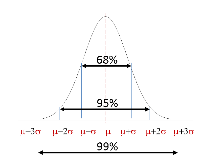
We can use the mean and standard deviation to get a handle on probability. It turns out that, as demonstrated in the figure below,
- Approximately 68% of values in the distribution are within 1 SD of the mean, i.e., above or below.
P (µ - σ < X < µ + σ) = 0.68
- Approximately 95% of values in the distribution are within 2 SD of the mean.
P (µ - 2σ < X < µ + 2σ) = 0.95
- Approximately 99% of values in the distribution are within 3 SD of the mean.
P (µ - 3σ < X < µ + 3σ) = 0.99
There are many variables that are normally distributed and can be modeled based on the mean and standard deviation. For example,
- BMI: µ=25.5, σ=4.0
- Systolic BP: µ=133, σ=22.5
- Birth Wgt. (gms) µ=3300, σ=500
- Birth Wgt. (lbs.) µ=7.3, σ=1.1
The ability to address probability is complicated by having many distributions with different means and different standard deviations. The solution to this problem is to project these distributions onto a standard normal distribution that will make it easy to compute probabilities.
The Standard Normal Distribution
The standard normal distribution is a special normal distribution that has a mean=0 and a standard deviation=1. This is very useful for answering questions about probability, because, once we determine how many standard deviations a particular result lies away from the mean, we can easily determine the probability of seeing a result greater or less than that.
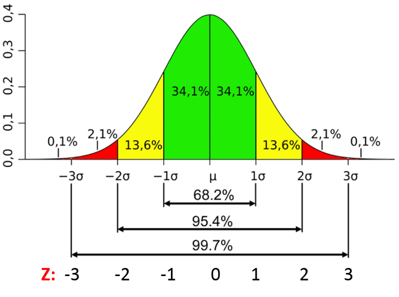
The figure below shows the percentage of observations that would lie within 1, 2, or 3 standard deviations from any mean in a distribution that is more or less normally distributed. For a given value in the distribution, the Z score is the number of standard deviations above or below the mean. We can think about probability from this.
- What is the probability of a value less than the mean? The obvious answer is 50%.
- What is the probability of a value less than I SD below the mean? P= 13.6+2.1+0.1=15.8%
- What is the probability of a value less than I SD above the mean? P= 34.1+34.1+13.6+2.1+0.1=84%
Example:
What is the probability of a Z score less than 0? Answer: P= 34.1+13.6+ 2.1+0.1=50%
What is the probability of a Z score less than +1? Answer: P= 34.1+34.1+13.6+2.1+0.1=84%
How many standard deviation units a given observation lies above or below the mean is referred to as a Z score, and there are tables and computer functions that can tell us the probability of a value less than a given Z score.
For example, in R:
> pnorm(0)
[1] 0.5
The probability of an observation less than the mean is 50%.
> pnorm(1)
[1] 0.8413447
The probability of an observation less than 1 standard deviation above the mean is 84.13%.
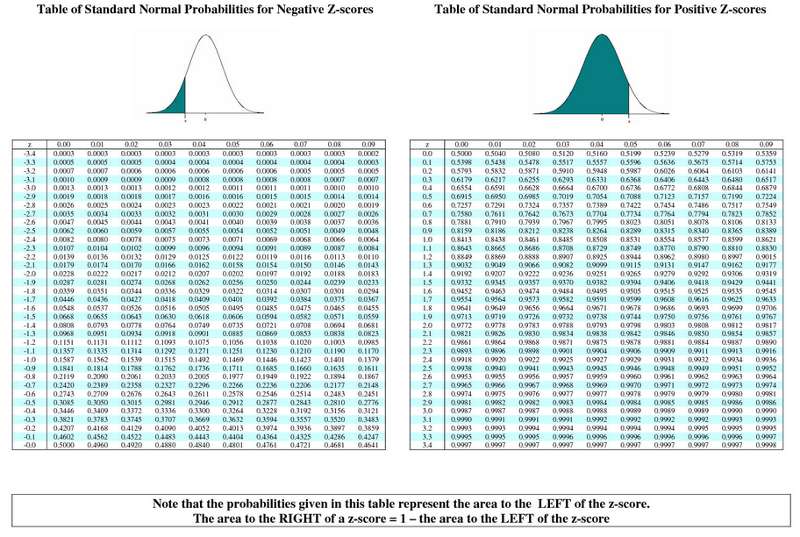
We can also look up the probability in a table of Z scores:
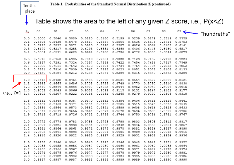
So, for any distribution that is more or less normally distributed, if we determine how many standard deviation units a given value is away from the mean (i.e., its corresponding Z score), then we can determine the probability of a value being less than or greater than that.
It is easy to determine how many SD units a value is from the mean of a normal distribution:

In other words, we determine how far a given value is from the mean and then divide that by the standard deviation to determine the corresponding Z score.
For example, BMI among 60 year old men is normally distributed with µ=29 and σ=6. What is the probability that a 60 year old male selected at random from this population will have a BMI less than 30? Stated another way, what proportion of the men have a BMI less than 30?
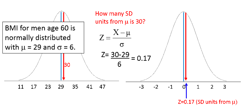
BMI=30 is just 0.17 SD units above the mean of 29. So, all we have to do is look up 0.17 in the table of Z scores to see what the probability of a value less than 30 is. Note that the table is set up in a very specific way. The entries in the middle of the table are areas under the standard normal curve BELOW the z score. The z score can be found by locating the units and tenths place along the left margin and the hundredths place across the top row.
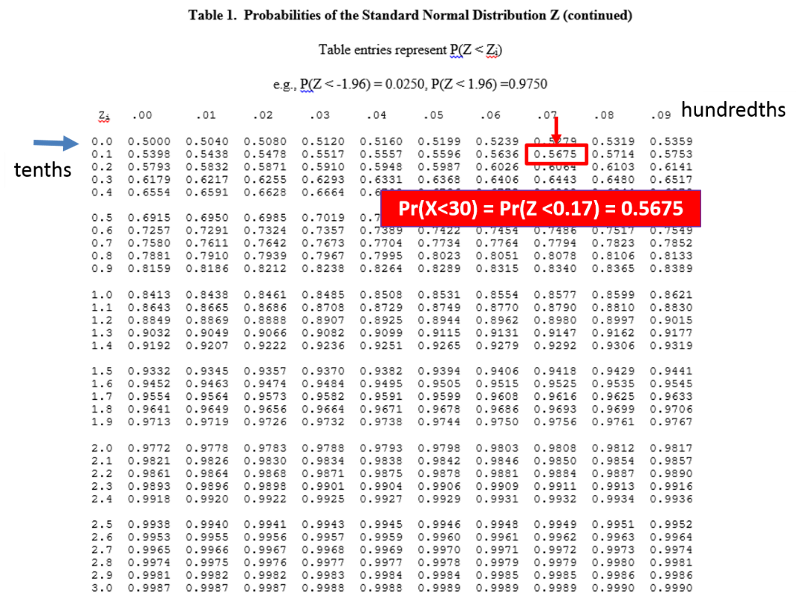
From the table of Z scores we can see that Z=0.17 corresponds to a probability of 0.5676.
We can also look up the probability using R:
>pnorm(0.17)
[1] 0.5674949
You can also have R automatically do the calculation of the Z score and look up the probability by using the pnorm function with the parameters (the value, the mean, and the standard deviation), e.g.:
# Use "pnorm(x,mean,SD)"
>pnorm(30,29,6)
[1] 0.5661838
The table of probabilities for the standard normal distribution gives the area (i.e., probability) below a given Z score, but the entire standard normal distribution has an area of 1, so the area above a Z of 0.17 = 1-0.5675 = 0.4325.
You can compute the probability above the Z score directly in R:
>1-pnorm(0.17)
[1] 0.4325051
A Slightly Different Example:
Now consider what the probability of BMI<30 would be in a slightly different population with the same mean (29), but less variability, with standard deviation=2. This distribution is narrower, so values less than 30 should represent a slightly greater proportion of the population.
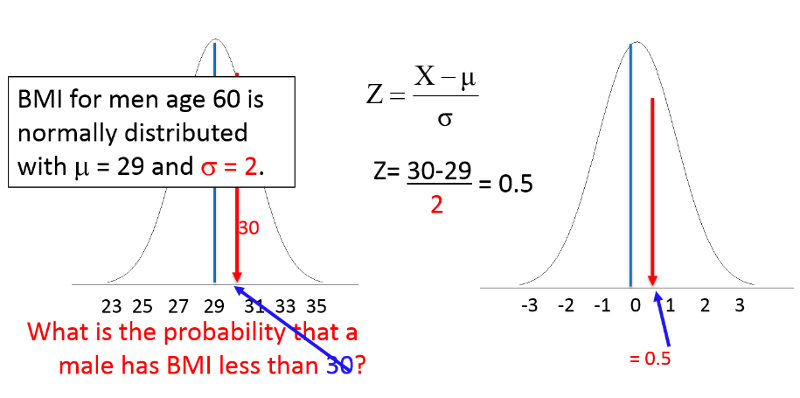
Using the same equation for Z:
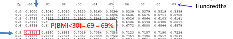
Conclusion: In this population 69% of men who are 60 years old will have BMI<30.
 Test Yourself
Problem #1
BMI among 60 year old men is normally distributed with µ=29 and σ=6. What is the probability that a 60 year old male selected at random from this population will have a BMI less than 40?
Problem #2
In the same population of 60 year old men with µ=29 and σ=6. What is the probability that a male age 60 has BMI greater than 40?
Problem #3
In the same population of 60 year old men with µ=29 and σ=6. What is the probability that a 60 year old male selected at random from this population will have a BMI between 30 and 40?
What if Z is a Negative Number?
Suppose I want to know what proportion of 60 year old men have BMI less than 25 in my population with µ=29 and σ=6. I compute the Z score as follows:
Z=(x-µ)/σ = (25-29)/6 = -0.6661
Here the value of interest is below the mean, so the Z score is negative. The full table of Z scores takes this into account as shown below. Note that the left page of the table has negative Z scores for values below the mean, and the page on the right has corresponding positive Z scores for values above the mean. In both cases the probability is the area to the left of the Z score.
If we use the left side of the table below and look up the probability for Z=-0.6661, the probability is about 0.2546.
Alternatively, we can use R to compute the probability as follows:
> pnorm(-0.666)
[1] 0.2527056