


Probability Distributions for Continuous Variables
So far, we have focused on dichotomous outcomes, i.e., outcomes that either occurred or did not occur. We will now turn our attention to outcome variables that are continuously distributed, such as BMI (body mass index), blood pressure, cholesterol, age, daily servings of alcohol, years of education, nutrient levels, height in inches, etc.
Suppose we measured the height in inches of 8,750 men in a population and created a frequency histogram of the proportion of men with specific heights, i.e., a probability distribution as shown in the figure below.
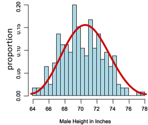
The distribution is reasonably bell-shaped (i.e., a normal distribution) with greater proportions of men in the middle of the distribution and smaller proportions as one moves from the center to the highest or lowest values. The shape of the distribution shows the degree of variability among the men; wider spread in the distribution means more variability.
If we add up all of the proportions, the sum has to be 1.0, so if we select a man at random, we can figure out the probability that his height will be more or less than a given number or even between two numbers by computing the area under the curve.
- What is the probability of observing a value higher (or lower) than a given height?
- Or, what proportion (or %) of observations are above or below a specific value?
For example, consider the table below that summarizes birth weights in a population of infants.
| Weight (lbs.) |
Relative Freq. (%) |
Cumulative Freq. (%) |
|
4.00-4.99 |
2.8 |
2.8% |
|
5.00-5.99 |
11.1 |
13.9% |
|
6.00-6.99 |
27.8 |
41.7% |
|
7.00-7.99 |
36.1 |
77.8% |
|
8.00-8.99 |
8.3 |
86.1% |
|
9.00-9.99 |
11.1 |
97.2% |
|
10.00-10.99 |
2.8 |
100% |
|
Total |
100 |
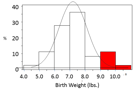
What is the probability that a given infant will have a birth weight greater than 9 lbs.?
The two birth weight categories at the bottom of the table meet this criterion, with 11.1% weighing between 9.00-9.99 lbs., and 2.8% weighing 10.00-10.99 lbs. So, the probability of a baby weight more than 9 lbs. is the sum of these or 13.9%.
Pr(X>9) = 11.1+2.8 = 13.9%
We could also visualize the answer if we presented these data as a probability distribution as shown in the histogram below.
Many, but not all, continuously distributed variables conform to a normal distribution (bell shaped), which is unimodal (it has one higher value) and more or less symmetric, i.e., the mean ≅ median ≅ mode. These distributions are characterized by their mean (μ, the lowercase Greek letter "mu") and their standard deviation (σ, the lowercase Greek letter "sigma"). The standard deviation is a measure of the variability in the distribution.
Consider the three distributions shown below. Which of these conforms to a reasonably normal distribution?
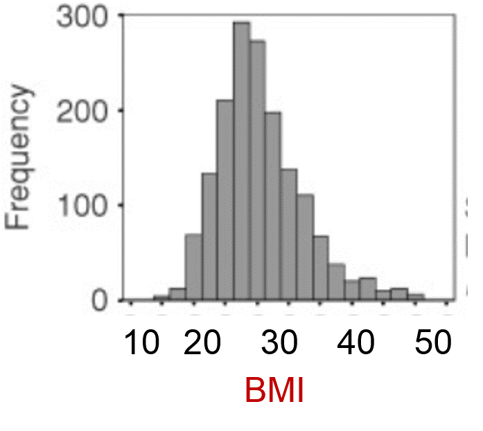
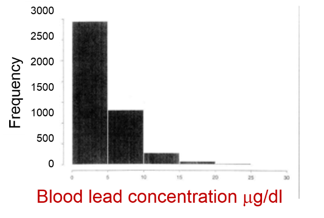
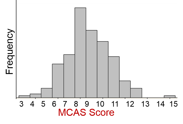
The distribution of blood lead levels is not normal; it is markedly skewed, since most people have low levels, although some have elevated levels. However, the distributions for BMI and MCAS scores are reasonably normal.
Models for Normally Distributed Variables: Normally distributed variables allow us to use models from which we can estimate probabilities without enumerating all possible outcomes, and this is very efficient. Since BMI is normally distributed, we could use a model to address questions like, "What is the probability of a BMI<30 in a population of 60 year old men?
Models for Dichotomous Variables: Dichotomous variables for outcomes that either occurred or did not occur can be described using the binomial distribution, which will not be covered in this course. These could be used to address some of the questions posed in the beginning of this module, such as:
- What is the probability a women with a positive screen test will have breast cancer?
- What is the probability that a baby born to a mother who is 40 years old will have Down syndrome?
