PH717 Module 6 - Random Error
Probability, Estimation, and Confidence Intervals

Introduction

Link to a Word file with the transcript of the video

Consider two examples in which samples are to be used to estimate some parameter in a population:

1. Suppose I wish to estimate the mean weight of the freshman class entering Boston University in the fall, and I select the first five freshmen who agree to be weighed. Their mean weight is 153 pounds. Is this an accurate estimate of the mean value for the entire freshman class? Intuitively, you know that the estimate might be off by a considerable amount, because the sample size is very small and may not be representative of the mean for the entire class. In addition, if I were to repeat this process and take multiple samples of five students and compute the mean for each of these samples, I would likely find that the estimates varied from one another by quite a bit. This also implies that some of the estimates are very inaccurate, i.e. far from the true mean for the class.
2. Suppose I have a box of marbles that are either blue or yellow, and I want you to estimate the proportion of blue marbles without looking into the box. I shake up the box and allow you to select 4 marbles and examine them to compute the proportion of blue marbles in your sample. Again, you know intuitively that the estimate might be very inaccurate, because the sample size is so small. If you were to repeat this process and take multiple samples of 4 marbles to estimate of the proportion of blue marbles, you would likely find that the estimates varied from one another by quite a bit, and many of the estimates would be very inaccurate.

The parameters being estimated differ in these two examples. The first is a measurement variable, i.e. body weight, which could have been any one of an infinite number of measurements on a continuous scale. In the second example the marbles are either blue or yellow (i.e., a discrete variable that can only have a limited number of values), and in each sample the proportion of blue marbles was determined in order to estimate the proportion of blue marbles in the entire box. Nevertheless, while these variables are of different types, they both illustrate the problem of random error when using a sample to estimate a parameter in a population.

The problem of random error also arises in epidemiologic investigations. The basic goals of epidemiologic studies are a) to measure a disease frequency or b) to compare measurements of disease frequency in two exposure groups in order to measure the extent to which there is an association with a health outcome. However, both of these estimates might be inaccurate because of random error.

Essential Questions

1. How do we differentiate differences that are real versus just due to chance?
2. How do we assess the uncertainty from samples?

Examples of Where This is Leading:

• Computing the probability of a continuous outcome :

• The BMIs in a population of 60 year-old men are normally distributed with μ = 29 and σ = 6. What is the probability of a man having BMI less than 30? (Note: μ denotes the mean of a variable in the population and σ is the standard deviation for that variable.)

• Determining whether groups differ with respect to a continuous measurement outcome:

• Do children born prematurely have lower IQs than average?
• Do patients randomized to a new drug have lower cholesterol levels than those receiving a placebo?
• A program to improve knowledge about HIV transmission was developed. Did the knowledge score of participants improve after going through the program?

Learning Objectives

After completing this section, you will be able to:

• Define the properties of a normal distribution
• Describe the relationship between the standard normal distribution and the Z-table
• Use the standard normal distribution to compute probabilities
• Define and distinguish between point estimate and confidence interval
• Define, calculate and interpret the 95% confidence interval for a mean and a proportion

What is Probability?

With regard to health outcomes probability is the proportion or percentage of events that occur in a group of people, i.e., the number of health outcomes or "events" divided by the total number of possible events.

Probabilities can be expressed as:

• A proportion from 0 to 1, e.g., 0.32 or
• A percentage, e.g., 0.32=32%

Example:

In the Physicians' Health Study on aspirin, male physicians were randomly assigned to take an aspirin or a placebo every other day. 

Test Yourself

Consider the data in the table below from the New York City Cancer Registry

(Selected data from http://www.health.state.ny.us/statistics/cancer/registry/about.htm)

What is the:

1. Probability that a cancer patient is a black male? [P(Black male)]
2. Probability that a cancer patient has thyroid cancer? [P(thyroid cancer)]
3. Probability that a cancer patient is a white female with liver cancer? [P(White female with liver cancer)]
4. Probability that a cancer patient is a black with lung cancer? [P(Black patient with lung cancer)]

Work these out yourself before looking at the answers.

 Answers

Conditional Probability

Conditional probability is the probability of an event occurring, given that another condition is true or another event has occurred.

Example: What proportion of patients with colorectal cancer are white?

Another way of stating this question is "Given that a patient has colorectal cancer, what is the probability that the patient is white?

The notation for this is P(white | colorectal cancer), where the "|" signals the condition. In this case, P(white | colorectal cancer) = (1236 + 1251)/3520 = 0.7065 = 71%. 

Test Yourself

Using the data in the table above:

1. What proportion of patients with leukemia are white?
2. What proportion of women have lung cancer?

Work these out yourself before looking at the answers.

Answers

Probability When Screening for Pre-clinical Disease

A basic understanding of probability is essential for interpreting screening tests for early disease. The validity of screening tests is evaluated by screening a large number of people and then evaluating the probability that the screen test correctly identified people with and without the disease by comparing the results to a more definitive determination of whether the disease was truly present or not. Sometimes the definitive answer is based on a more extensive battery of diagnostic tests, and sometimes it is determined by simply waiting to see if the disease occurs within a certain follow up period of time.

Results from an evaluation of a screening test are summarized in a different type of contingency table as shown in the table below showing results for a screening test for breast cancer in 64,810 women. 

There were 177 women who were ultimately found to have had breast cancer, and 64,633 women remained free of breast cancer during the observation period. Among the 177 women with breast cancer, 132 had a positive screening test (true positives), but 45 of the women with breast cancer had negative tests (false negatives). Among the 64,633 women without breast cancer, 63,650 appropriately had negative screening tests (true negatives), but 983 incorrectly had positive screening tests (false positives).

If we focus on the rows, we find that 1,115 subjects had a positive screening test, i.e., the screening results were abnormal and suggested disease. However, only 132 of these were found to actually have disease. Also note that 63,695 people had a negative screening test, suggesting that they did not have the disease, but, in fact 45 of these people were actually diseased.

Sensitivity of a Screening Test

One measure of test validity is sensitivity, i.e., the probability of a positive screening test in people who truly have the disease. When thinking about sensitivity, focus on the individuals who really were diseased - in this case, the left-hand column.

Table - Sensitivity of a Screening Test

The probability of a positive screening test in women who truly have breast cancer is:

P(Screen+ | breast cancer) = 132/177 = 0.746 = 74.6%.

Interpretation: "The probability of the screening test correctly identifying women with breast cancer was 74.6%."

Specificity of a Screening Test

Specificity focuses on the probability that non-diseased subjects will be classified as non-diseased by the screening test. Now we focus on the column for women who were truly not diseased.

Table - Specificity of a Screening Test

 The probability of a positive screening test in women who truly have breast cancer is:

P(Screen- | no breast cancer) = 63,650/64,633 = 0.985 = 98.5%.

Interpretation: "The probability of the screening test correctly identifying women without breast cancer was 98.5%."

Test Yourself

In the above example, what was the prevalence of disease among the 64,810 women in the study population? Compute the answer on your own before looking at the answer.

Answer

Positive and Negative Predictive Value of a Screening Test

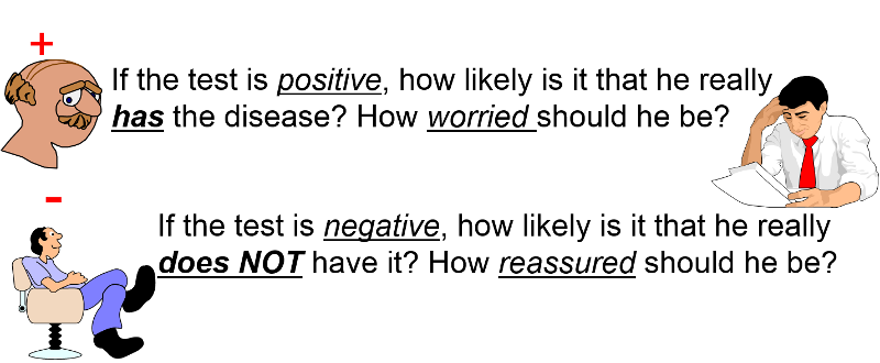
Another way of thinking about the same results is from the patient's point of view after receiving the results of their screening test. Consider men who are getting the results of a blood test that is used as a screening test for prostate cancer (the PSA test [prostate specific antigen]). If the screening test was positive, what is the probability that they really have cancer; how worried should they be? Conversely, if a patient is told that his prostate cancer screening test was negative, how reassured should she be?

Positive Predictive Value

If a test subject has an abnormal screening test (i.e., it's positive), what is the probability that the subject really has the disease?  Now, we shift our focus to the first row in the contingency table we have been using.

Table - Positive Predicative Value Focuses on the First Row

There were 1,115 women with positive screening tests, but only 132 of these actually had the disease. Therefore, even if a subject's screening test was positive, the probability of actually having breast cancer was:

P(breast cancer | Screen+) = 132/1,115 = 11.8%

Interpretation: Among those who had a positive screening test, the probability of disease was 11.8%.

Negative Predictive Value

If a test subject has a negative screening test, what is the probability that she doesn't have breast cancer? In our example, there were 63,695 subjects whose screening test was negative, and 63,650 of these were, in fact, free of disease. Now we focus on the "test negative" row in the contingency table.

Table - Negative Predicative Value

 The negative predictive value is:

P(no breast cancer | Screen-) = 63,650/63,950=0.999, or 99.9%.

Interpretation: Among those who had a negative screening test, the probability of being disease-free was 99.9%.

Test Yourself

Problem #1

A group of women aged 40 are screened for breast cancer, and 1% of these women will have breast cancer. 80% of women with breast cancer will have a positive mammogram, while 9.6% of women without breast cancer will have a positive mammogram.

What is the probability that a woman with a positive mammogram has breast cancer? [Hint: Using the information provided, create a contingency table based on a total of 10,000 screened women, and use the percentages to derive the number of subjects in each category.]

Answer in Word file

Problem #2

Computed tomography (CT) scans are used as a screening test for lung cancer. The test involves X-ray at low doses of radiation to take detailed images of the lungs. The images are read by a radiologist and classified as needing further clinical examination or not. Diagnostic tests for lung cancer are based on sputum cytology and evaluated by a certified cytopathologist. 

A study was done in which 1200 persons aged 55 to 80 years who currently smoke or quit within the past 15 years and have at least a 30-pack-year history of cigarette smoking underwent both CT scans (as a possible screening test) and sputum cytology (as a diagnostic test). CT scans were read and classified as needing further clinical examination (screen positive) or not (screen negative). Analysis of sputum cytology indicated whether the patient actually had a lung cancer or not. The results are summarized in the table below.

Compute the sensitivity, specificity, false negative fraction, false positive fraction, the positive predictive value, and the negative predictive value of the CT as a screening test for lung cancer.

Link to Answers in a Word file

Is this a good screening test for lung cancer?

US Preventative Services Task Force Recommendations

Probability Distributions for Continuous Variables

So far, we have focused on dichotomous outcomes, i.e., outcomes that either occurred or did not occur. We will now turn our attention to outcome variables that are continuously distributed, such as BMI (body mass index), blood pressure, cholesterol, age, daily servings of alcohol, years of education, nutrient levels, height in inches, etc.

Suppose we measured the height in inches of 8,750 men in a population and created a frequency histogram of the proportion of men with specific heights, i.e., a probability distribution as shown in the figure below.

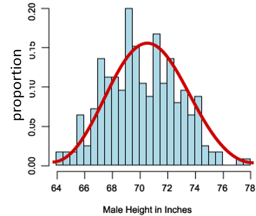
The distribution is reasonably bell-shaped (i.e., a normal distribution) with greater proportions of men in the middle of the distribution and smaller proportions as one moves from the center to the highest or lowest values. The shape of the distribution shows the degree of variability among the men; wider spread in the distribution means more variability.

If we add up all of the proportions, the sum has to be 1.0, so if we select a man at random, we can figure out the probability that his height will be more or less than a given number or even between two numbers by computing the area under the curve.

• What is the probability of observing a value higher (or lower) than a given height?
• Or, what proportion (or %) of observations are above or below a specific value?

For example, consider the table below that summarizes birth weights in a population of infants.

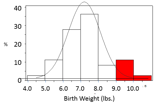
What is the probability that a given infant will have a birth weight greater than 9 lbs.?

The two birth weight categories at the bottom of the table meet this criterion, with 11.1% weighing between 9.00-9.99 lbs., and 2.8% weighing 10.00-10.99 lbs. So, the probability of a baby weight more than 9 lbs. is the sum of these or 13.9%.

Pr(X>9) = 11.1+2.8 = 13.9%

We could also visualize the answer if we presented these data as a probability distribution as shown in the histogram below.

Many, but not all, continuously distributed variables conform to a normal distribution (bell shaped), which is unimodal (it has one higher value) and more or less symmetric, i.e., the mean ≅ median ≅ mode. These distributions are characterized by their mean (μ, the lowercase Greek letter "mu") and their standard deviation (σ, the lowercase Greek letter "sigma"). The standard deviation is a measure of the variability in the distribution.

Consider the three distributions shown below. Which of these conforms to a reasonably normal distribution?

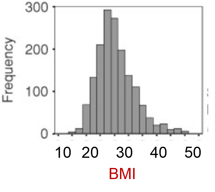
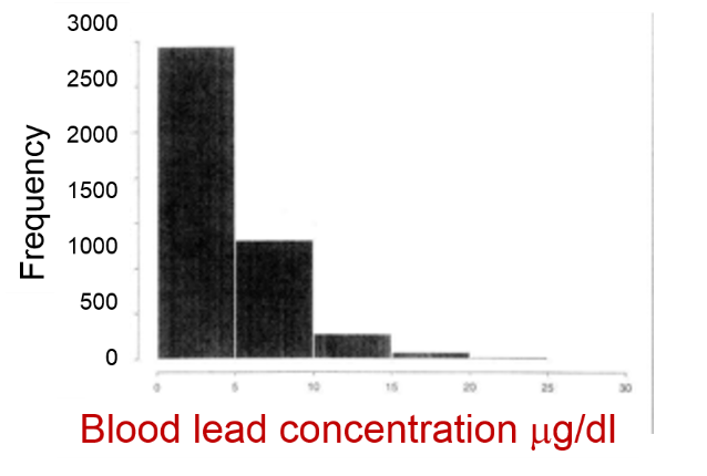
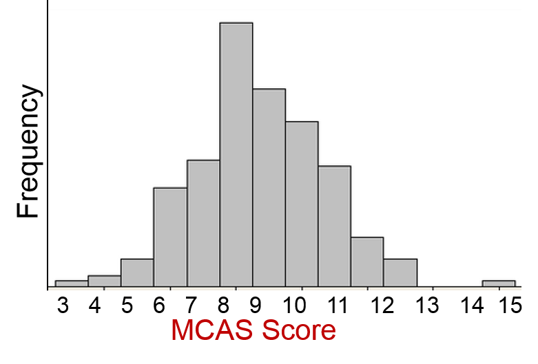
The distribution of blood lead levels is not normal; it is markedly skewed, since most people have low levels, although some have elevated levels. However, the distributions for BMI and MCAS scores are reasonably normal.

Models for Normally Distributed Variables: Normally distributed variables allow us to use models from which we can estimate probabilities without enumerating all possible outcomes, and this is very efficient. Since BMI is normally distributed, we could use a model to address questions like, "What is the probability of a BMI<30 in a population of 60 year old men?

Models for Dichotomous Variables: Dichotomous variables for outcomes that either occurred or did not occur can be described using the binomial distribution, which will not be covered in this course. These could be used to address some of the questions posed in the beginning of this module, such as:

• What is the probability a women with a positive screen test will have breast cancer?
• What is the probability that a baby born to a mother who is 40 years old will have Down syndrome?

Characteristics of a Normal Distribution

In our earlier discussion of descriptive statistics, we introduced the mean as a measure of central tendency and variance and standard deviation as measures of variability. We can now use these parameters to answer questions related to probability.

For a normally distributed variable in a population the mean is the best measure of central tendency, and the standard deviation(s) provides a measure of variability.

The notation for a sample from a population is slightly different:

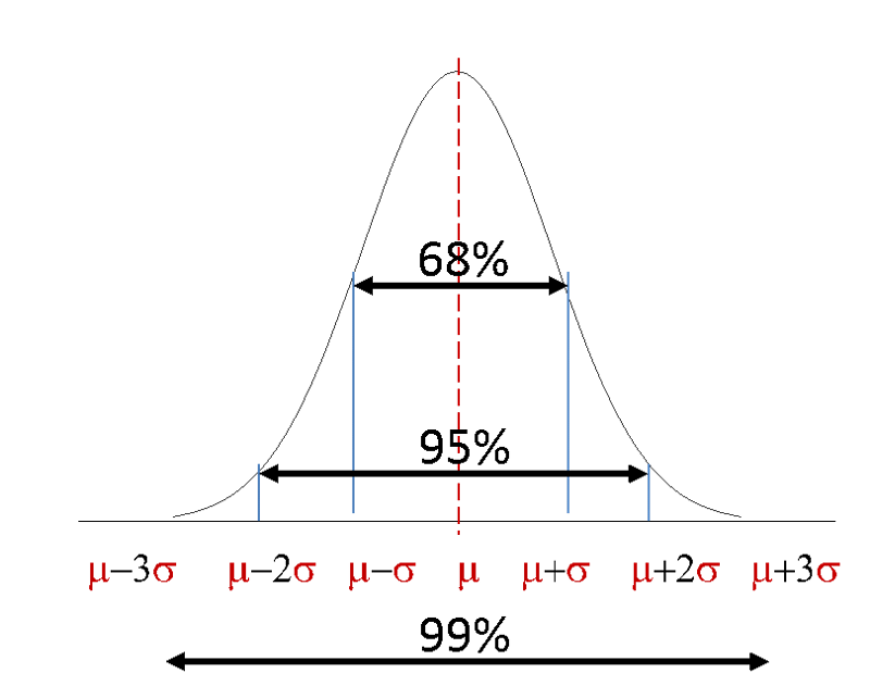
We can use the mean and standard deviation to get a handle on probability. It turns out that, as demonstrated in the figure below,

• Approximately 68% of values in the distribution are within 1 SD of the mean, i.e., above or below.

  P (µ - σ < X < µ + σ) = 0.68

• Approximately 95% of values in the distribution are within 2 SD of the mean.

  P (µ - 2σ < X < µ + 2σ) = 0.95

• Approximately 99% of values in the distribution are within 3 SD of the mean.

  P (µ - 3σ < X < µ + 3σ) = 0.99

There are many variables that are normally distributed and can be modeled based on the mean and standard deviation. For example,

• BMI: µ=25.5, σ=4.0
• Systolic BP: µ=133, σ=22.5
• Birth Wgt. (gms) µ=3300, σ=500
• Birth Wgt. (lbs.) µ=7.3, σ=1.1

The ability to address probability is complicated by having many distributions with different means and different standard deviations. The solution to this problem is to project these distributions onto a standard normal distribution that will make it easy to compute probabilities.

The Standard Normal Distribution

The standard normal distribution is a special normal distribution that has a mean=0 and a standard deviation=1. This is very useful for answering questions about probability, because, once we determine how many standard deviations a particular result lies away from the mean, we can easily determine the probability of seeing a result greater or less than that.

The figure below shows the percentage of observations that would lie within 1, 2, or 3 standard deviations from any mean in a distribution that is more or less normally distributed. For a given value in the distribution, the Z score is the number of standard deviations above or below the mean. We can think about probability from this.

• What is the probability of a value less than the mean? The obvious answer is 50%.
• What is the probability of a value less than I SD below the mean?  P= 13.6+2.1+0.1=15.8%
• What is the probability of a value less than I SD above the mean?  P= 34.1+34.1+13.6+2.1+0.1=84%

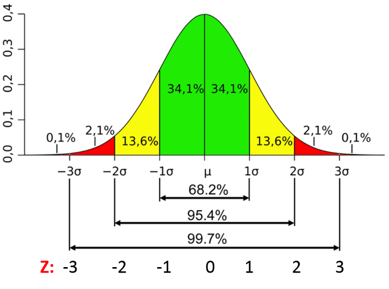
Example:
What is the probability of a Z score less than 0?   Answer: P= 34.1+13.6+  2.1+0.1=50%
What is the probability of a Z score less than +1? Answer: P= 34.1+34.1+13.6+2.1+0.1=84%

How many standard deviation units a given observation lies above or below the mean is referred to as a Z score, and there are tables and computer functions that can tell us the probability of a value less than a given Z score.

For example, in R:

> pnorm(0)
[1] 0.5

The probability of an observation less than the mean is 50%.

> pnorm(1)
[1] 0.8413447

The probability of an observation less than 1 standard deviation above the mean is 84.13%.

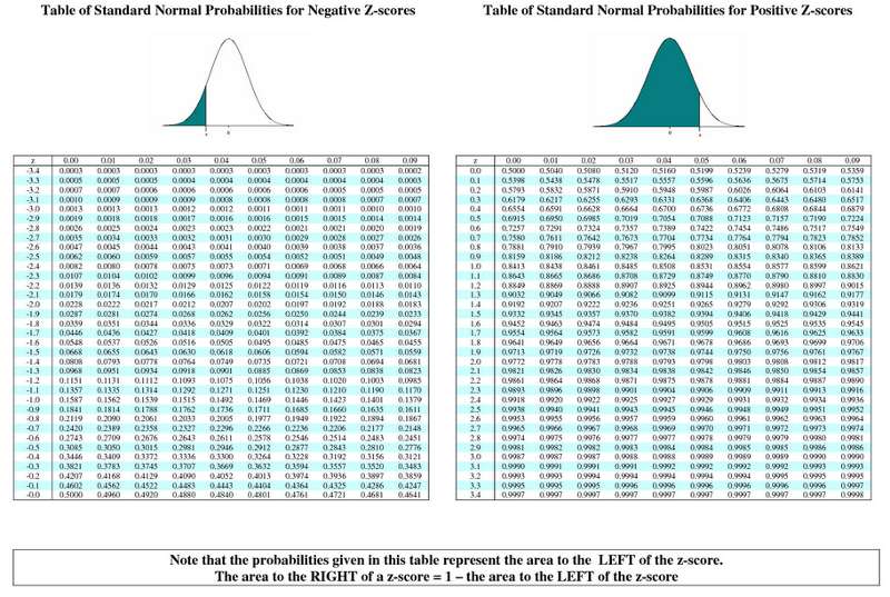
We can also look up the probability in a table of Z scores:

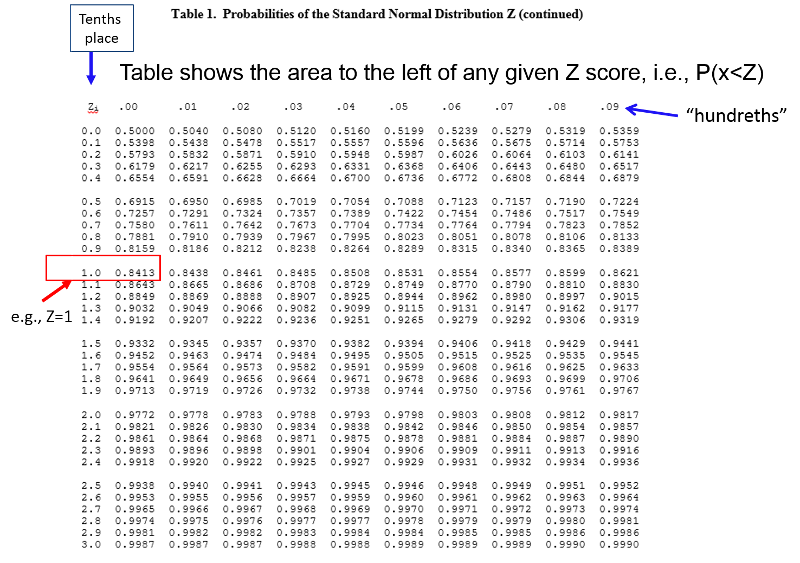
So, for any distribution that is more or less normally distributed, if we determine how many standard deviation units a given value is away from the mean (i.e., its corresponding Z score), then we can determine the probability of a value being less than or greater than that.

It is easy to determine how many SD units a value is from the mean of a normal distribution:

In other words, we determine how far a given value is from the mean and then divide that by the standard deviation to determine the corresponding Z score.

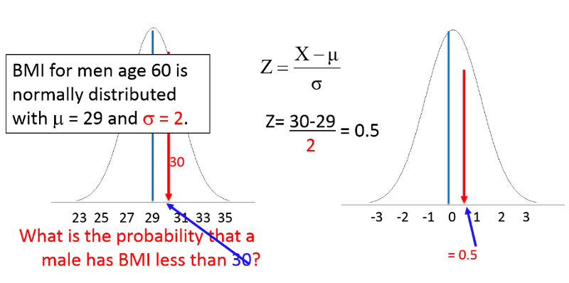
For example, BMI among 60 year old men is normally distributed with µ=29 and σ=6. What is the probability that a 60 year old male selected at random from this population will have a BMI less than 30? Stated another way, what proportion of the men have a BMI less than 30?

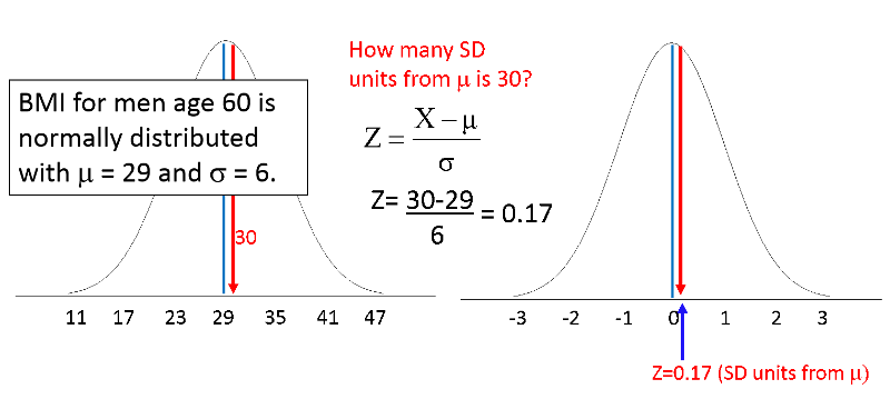
BMI=30 is just 0.17 SD units above the mean of 29. So, all we have to do is look up 0.17 in the table of Z scores to see what the probability of a value less than 30 is. Note that the table is set up in a very specific way. The entries in the middle of the table are areas under the standard normal curve BELOW the z score. The z score can be found by locating the units and tenths place along the left margin and the hundredths place across the top row.

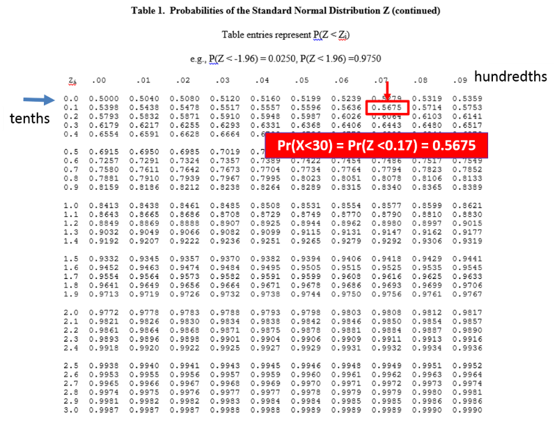
From the table of Z scores we can see that Z=0.17 corresponds to a probability of 0.5676.

We can also look up the probability using R:

>pnorm(0.17)
[1] 0.5674949

You can also have R automatically do the calculation of the Z score and look up the probability by using the pnorm function with the parameters (the value, the mean, and the standard deviation), e.g.:

# Use "pnorm(x,mean,SD)"
>pnorm(30,29,6)
[1] 0.5661838

The table of probabilities for the standard normal distribution gives the area (i.e., probability) below a given Z score, but the entire standard normal distribution has an area of 1, so the area above a Z of 0.17 = 1-0.5675 = 0.4325.

You can compute the probability above the Z score directly in R:

>1-pnorm(0.17)
[1] 0.4325051

A Slightly Different Example:

Now consider what the probability of BMI<30 would be in a slightly different population with the same mean (29), but less variability, with standard deviation=2. This distribution is narrower, so values less than 30 should represent a slightly greater proportion of the population.

Using the same equation for Z:

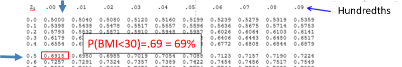
Conclusion: In this population 69% of men who are 60 years old will have BMI<30.

Test Yourself

Problem #1

BMI among 60 year old men is normally distributed with µ=29 and σ=6. What is the probability that a 60 year old male selected at random from this population will have a BMI less than 40?

Answer

Problem #2

In the same population of 60 year old men with µ=29 and σ=6. What is the probability that a male age 60 has BMI greater than 40?

Answer

Problem #3

In the same population of 60 year old men with µ=29 and σ=6. What is the probability that a 60 year old male selected at random from this population will have a BMI between 30 and 40?

Answer in a Word file

What if Z is a Negative Number?

Suppose I want to know what proportion of 60 year old men have BMI less than 25 in my population with µ=29 and σ=6. I compute the Z score as follows:

Z=(x-µ)/σ = (25-29)/6 = -0.6661

Here the value of interest is below the mean, so the Z score is negative. The full table of Z scores takes this into account as shown below. Note that the left page of the table has negative Z scores for values below the mean, and the page on the right has corresponding positive Z scores for values above the mean. In both cases the probability is the area to the left of the Z score.

If we use the left side of the table below and look up the probability for Z=-0.6661, the probability is about 0.2546.

Alternatively, we can use R to compute the probability as follows:

> pnorm(-0.666)
[1] 0.2527056

Z-scores as Summary Measures

The standard normal distribution also provides a "standardized" way of comparing individuals from two different normal distributions. For example, suppose we have two boys, a 12 month old who is 80 cm. tall and a 15 month old who is 82 cm. tall. Which one is taller for his age?

• Heights of 12 month-old boys are normally distributed with μ=76.4 cm. and σ=2.9
• Heights of 15 month-old boys are also normally distributed with μ=79.4 cm. and σ=3.2

An easy way to make a standardized comparison is to compute each boy's Z score, i.e., how many standard deviations their height is from the mean.

For the 12 month old: Z_{12 mo.} = (80-76.4)/2.9 = 1.24
For the 12 month old: Z_{15 mo.} = (82-79.4) / 3.2 = 0.81

Both boys are above average height (because both Z > 0), but the 12 month old is taller for his age than the 15 month old.

Finding Percentiles with the Normal Distribution

A percentile is the value in a normal distribution that has a specified percentage of observations below it. Percentiles are often used in standardized tests like the GRE and in comparing height and weight of children to gauge their development relative to their peers. The table below shows a portion of the percentile ranks for verbal and quantitative scores on the GRE exam. For example, if you scored 166 on the quantitative reasoning portion of the GRE, then 91% of those who took the test scored lower than you. If your score was 153, then 51% of those taking the exam scored lower than you.

We might ask, "In a population of 60 year old men with a mean BMI = 29 and s=6, what is the 90^th percentile for BMI?"

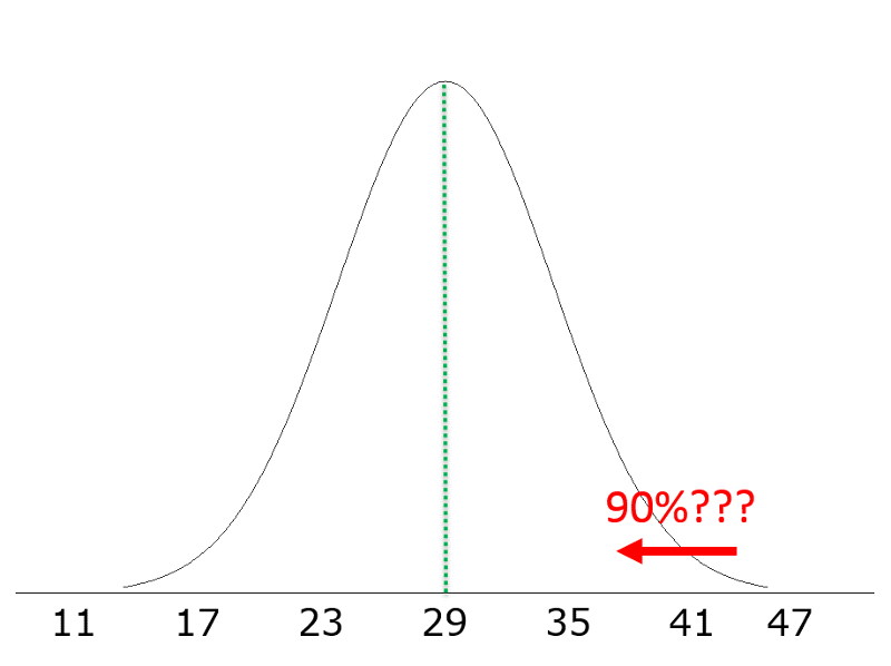
Previously, we started with a value, and asked what was the probability of values less (or greater) than that. However, we are now asking a problem that runs in the other direction. We are given the proportion or probability (90^th percentile) and asked what value of BMI that corresponds to.

Consequently, we use the previous concept and equation, but we work backwards.

First, we go the Z table and find the probability closest to 0.90 and determine what the corresponding Z score is.

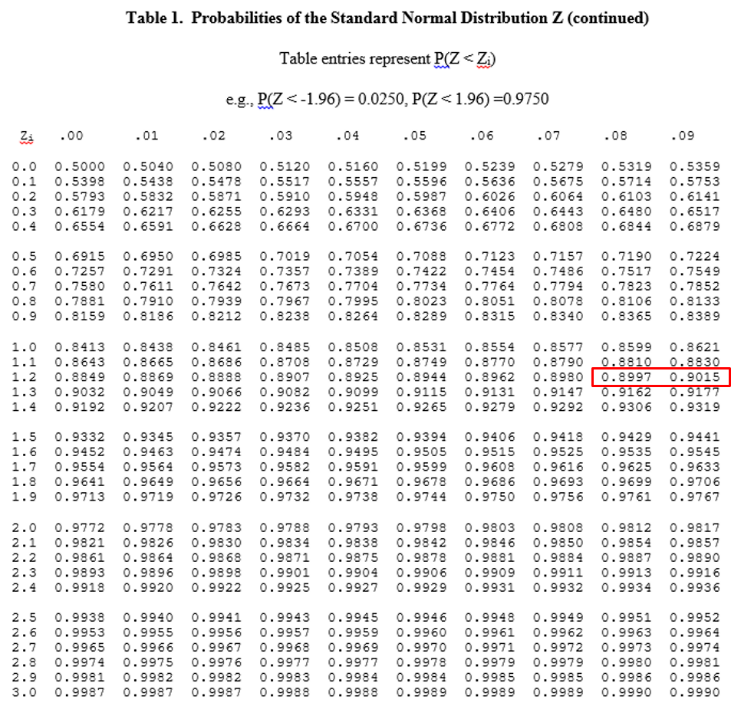
For any normal distribution a probability of 90% corresponds to a Z score of about 1.28.

We also could have computed this using R by using the qnorm() function to find the Z score corresponding to a 90 percent probability.

> qnorm(0.90)
[1] 1.281552

So, given a normal distribution with μ =29 and σ =6, what value of BMI corresponds to a Z score of 1.28?

We know that Z=(x-μ)/σ.

Previously, we knew x, μ, and σ and computed Z. Now, we know Z, μ, and σ, and we need to compute X, the value corresponding to the 90^th percentile for this distribution. We can do this by rearranging the equation to solve for "x".

 x = μ + Z σ

In this case, x = 29 + 1.28(6) = 36.7

Conclusion: 90% of 60 year old men have BMI values less than 36.7.

Test Yourself

The height of 12 month old boys is normally distributed with μ=76.4, σ=2.9 cm. What is the 10^th percentile for height?

Answer

Variability in Means Obtained from a Sample

So far, we have been discussing the probability that a person or persons will have a value less than or greater than a certain value, but now we are shifting gears and building on those concepts. Instead of asking about the probable results when we select a random person from a normally distributed population, we will now consider the situation when we are selecting a random sample from a population to estimate a mean.

The standard deviation provided a measure of variability among individuals within the population, but now we need to address the issue of variability in the estimates of means obtained from samples of individuals.

Let's go back to our normally distributed population of 60 year old men. If I were to take one sample, I could compute an estimate of the mean and the SD of the population, and if the sample were large, I would probably get estimates close to the true mean and SD of the entire population.

However, if I were to take multiple samples (e.g., n=10 in each sample) and computed the mean of each sample, the means would also conform to a normal distribution. In the image below the outermost bell-shaped curve represents the distribution of individual BMI measurements among the men in the population. This distribution has a mean of 29 and SD=6.

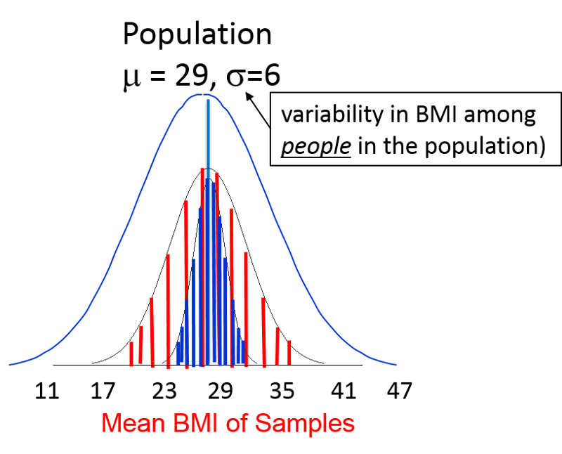
The mean of the sample means would be very close to μ, the mean for the population from which the samples were drawn. However, the variability in the sample means will depend on the size of the samples, since larger samples are more likely to give estimated means that are closer to the true mean of the population. In the figure above, the vertical red lines represent the distribution of means obtained with samples of n=10. The vertical blue lines represent the distribution of sample means that might be obtained with a larger sample, say n=30. Therefore, the variability in the sample means depends on the sample size, and it turns out that the variability in sampling means can be estimated as follows:

In the example above the standard deviation was 6. If we took a sample of 10 subjects, the standard error of the mean would be as follows:

However, if we took a sample size of n=50, then the SE becomes smaller.

So, as the sample size increases, we obtain greater precision in the estimated mean.

We should also note that we almost never know the true mean and standard deviation of the population, but we can estimate the standard deviation in the population from the standard deviation in the sample, because the variability in individual measurements within a sample will be similar to the individual variability in the overall population. So, I can use the SD of a sample to estimate the SD of the population, and I will use this estimate of population SD to compute the SE, which is the standard deviation of the sample mean (SE).

The Probability of a Sample Mean

We saw in the previous section that if we take samples, the distribution of the sample means will be approximately normal. This will hold true even when the underlying population is not normally distributed, provided we take samples of n=30 or greater. If the population is normally distributed, the sample means will be normally distributed even with smaller samples. [This is known as the Central Limit Theorem, which states that when a large number of random samples are drawn from a population, the means of these samples will be normally distributed.]

Since the sample means are normally distributed, we can use Z scores to compute probabilities with respect to means.

Note that earlier in our discussion we were using Z scores to compute probabilities for values among individuals in a population, using the equation:

Now we are shifting to a new type of questions regarding the probability of obtaining means in samples drawn from a population. Since sampling means are normally distributed, we can use a modified version of the equation above:

With this new tool, let's go back to the population of 60 year old men with mean BMI, μ =29 and σ =6, and take multiple samples of n=40 men. What is the  probability that the mean BMI will be <30 if BMI μ=29 , σ=6? In other words, what percentage of possible samples would have mean BMI <30, if μ=29 and σ=6? Remember that even though the population we are sampling has individual variability of σ=6, the distribution for the sampling means is the standard error (σ/√n)

First, we use the equation:

And then we look up the probability for this Z score from the table, or we can use R as follows:

> pnorm(1.05)
[1] 0.8531409

So, the probability that the mean BMI of the samples is <30 is 85%.

Test Yourself

Problem #1

Total cholesterol in children aged 10-15 is assumed to follow a normal distribution with a mean of 191 and a standard deviation of 22.4. What proportion of children 10-15 years of age would be classified as hyperlipidemic (defined as a total cholesterol level over 200)?

Link to Answer in a Word file

Problem #2

Same scenario as the previous question. Total cholesterol in children aged 10-15 is assumed to follow a normal distribution with a mean of 191 and a standard deviation of 22.4. A sample of 20 children is selected. What is the probability that the mean cholesterol level of the sample will be > 200?

Link to Answer in a Word file

Problem #3

Same scenario: Total cholesterol in children aged 10-15 is assumed to follow a normal distribution with a mean of 191 and a standard deviation of 22.4. What proportion of children 10-15 years of age have total cholesterol between 180-190?

Link to Answer in a Word file

Confidence in Our Estimates

We almost never know the true parameters in a population (e.g., a population mean, a population proportion, a risk ratio, a risk difference, an odds ratio, etc.), and our goal is to make valid inferences about population parameters based on a single random sample from the population.

There are two types of estimates for population parameters:

1. A point estimate for a population parameter is the best estimate of that parameter based on a sample, but having estimated a parameter, such as a mean, how confident are we that the estimate reflects the true parameter in the population?
2. A confidence interval is a range of plausible values for the population parameter with a level of confidence attached (e.g., 95% confidence that the range or interval contains the parameter).

To address this we must calculate and interpret confidence intervals for

• means
• and proportions,
• risk ratios,
• odds ratios,
• etc.

Example: A team was assembled to estimate the mean waiting time (in minutes) in the Emergency Room (ER) of a particular suburban hospital during weekends. Two members of the team recorded a sample of waiting times from which they submitted estimates of the mean waiting time.

Sample #1: Was based on a sample of wait times for 100 random patients in the ER on weekends, and found a mean waiting time of X = 37.85 minutes to see a medical care provider. This is the point estimate.

Sample #2: The 2nd investigator based her estimate on a sample off 35 patients in the ER during weekends and found a mean waiting time of X = 33.75 minutes. (A second point estimate)
Which estimate is better, i.e., more accurate?

If by "more accurate" we mean closer to the true mean waiting time, we can't really tell. However, intuitively you know that the larger sample is more likely to be close to the true mean, and the notion that the larger sample is more likely to provide a better estimate is consistent with the Central Limit Theorem, since the larger sample will provide an estimate with a narrower standard error (SE). We are more confident in the larger sample.

The 95% Confidence Interval for Mean

A frequently used convention is to report the 95% confidence interval for a mean, i.e., the range within which the true mean is likely to lie, with 95% confidence.

Consider a normal distribution. The range of Z scores that would likely capture 95% of the observations would be the 95% of Z scores in the middle of the standard normal distribution, i.e., excluding the 2.5% of the Z scoress at the bottom of the standard normal distribution and the 2.5% of Z scores at the top. The Z-scores for these upper and lower limits for a 95% confidence interval are:

> qnorm(0.025)
[1] -1.959964
> qnorm(0.975)
[1] 1.959964

In other words, 95% of the observations will lie within Z= -1.96 to Z= 1.96 as shown in the figure below.

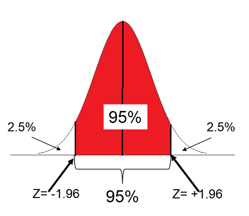
So, when estimating a mean with a large sample (>30), the 95% confidence interval for a point estimate is:

Point estimate ± 1.96(SE)

Where 1.96 (SE) is the "margin of error."

Now, back to the studies of waiting times in the ER:

• The first ER waiting room time study had a point estimate of 37.85 minutes with a sample of n=100. The 95% confidence interval for the mean waiting time is:

Therefore, the 95% confidence interval is: (35.99 to 39.71)

Interpretation:  Mean waiting time in the first sample was 37.85 minutes. We are 95% confident that the true mean waiting time in the ER is between 35.99 and 39.71 minutes. (margin of error = 1.86 minutes)

• The second point estimate was 33.75 with a sample of n=35. The 95% confidence interval:

Therefore, the 95% confidence interval is: (30.60, 36.90)

The first interval has a width of 3.71, and the second one has a width of 6.3, so the first one with the larger sample size is narrower and provides a more precise estimate of the true mean.

What the Confidence Interval Really Means

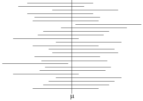
Strictly speaking, what the 95% confidence interval really means is that if we took a very large number of random samples of the same sample size and computed the mean and 95% confidence interval for each, about 95% of them would contain the true mean in the population from which the samples were drawn. In the figure below the true mean is shown with a vertical line; the many horizontal lines represent the 95% confidence intervals that were computed when many samples where taken to estimate the mean. The confidence intervals are all the same width, because the same sample size was used, but the confidence are not all centered on the true mean. They vary in position because the means that were obtained varied. However, about 95% of the confidence intervals included the true mean.

Other Confidence Intervals

A 95% confidence interval is most commonly used in biomedical and health sciences, but one can easily compute confidence intervals of any width just by selecting the appropriate Z score for the desired interval. The table below shows the Z scores that one would use for a specified confidence interval. The 95% confidence interval, which corresponds to a Z score of 1.96, is highlighted in red because it is the most commonly used confidence interval in the biomedical literature.

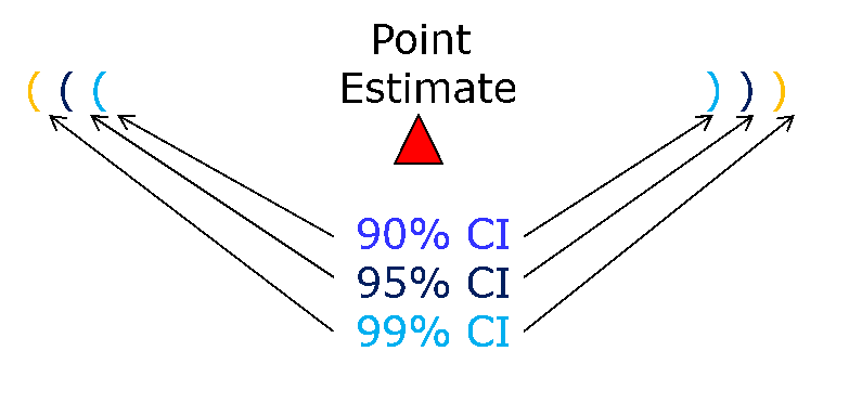
Also note that the confidence interval's width increases as the degree of confidence increases. For example, for a given sample a 99% confidence interval is always wider than the 95% confidence interval since it must "cast a wider net" in order to have a better chance of capturing the true value.

Confidence Intervals for Sample Size Less Than 30

In the preceding discussion we have been using s, the population standard deviation, to compute the standard error. However, we don't really know the population standard deviation, since we are working from samples. To get around this, we have been using the sample standard deviation (s) as an estimate. This is not a problem if the sample size is 30 or greater because of the central limit theorem. However, if the sample is small (<30) , we have to adjust and use a t-value instead of a Z score in order to account for the smaller sample size and using the sample SD.  

Therefore, if n<30, use the appropriate t score instead of a z score, and note that the t-value will depend on the degrees of freedom (df) as a reflection of sample size. When using the t-distribution to compute a confidence interval, df = n-1.

Calculation of a 95% confidence interval when n<30 will then use the appropriate t-value in place of Z in the formula:

The T-distribution

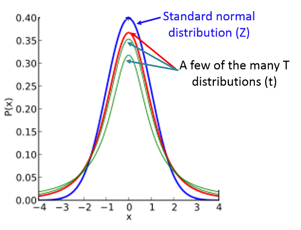
One way to think about the t-distribution is that it is actually a large family of distributions that are similar in shape to the normal standard distribution, but adjusted to account for smaller sample sizes. A t-distribution for a small sample size would look like a squashed down version of the standard normal distribution, but as the sample size increase the t-distribution will get closer and closer to approximating the standard normal distribution.

The table below shows a portion of the table for the t-distribution. Notice that sample size is represented by the "degrees of freedom" in the first column. For determining the confidence interval df=n-1. Notice also that this table is set up a lot differently than the table of Z scores. Here, only five levels of probability are shown in the column titles, whereas in the table of Z scores, the probabilities were in the interior of the table. Consequently, the levels of probability are much more limited here, because t-values depend on the degrees of freedom, which are listed in the rows.  

Notice that the value of t is larger for smaller sample sizes (i.e., lower df). When we use "t" instead of "Z" in the equation for the confidence interval, it will result in a larger margin of error and a wider confidence interval reflecting the smaller sample size.

With an infinitely large sample size the t-distribution and the standard normal distribution will be the same, and for samples greater than 30 they will be similar, but the t-distribution will be somewhat more conservative. Consequently, one can always use a t-distribution instead of the standard normal distribution. However, when you want to compute a 95% confidence interval for an estimate from a large sample, it is easier to just use Z=1.96.

Because the t-distribution is, if anything, more conservative, R relies heavily on the t-distribution.

 Test Yourself

Problem #1

Using the table above, what is the critical t score for a 95% confidence interval if the sample size (n) is 11?

Answer

Problem #2

A sample of n=10 patients free of diabetes have their body mass index (BMI) measured. The mean is 27.26 with a standard deviation of 2.10. Generate a 90% confidence interval for the mean BMI among patients free of diabetes.

Link to Answer in a Word file

Confidence Intervals for a Mean Using R

Instead of using the table, you can use R to generate t-values. For example, to generate t values for calculating a 95% confidence interval, use the function qt(1-tail area,df).

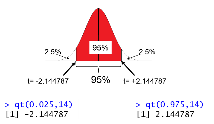
For example, if the sample size is 15, then df=14, we can calculate the t-score for the lower and upper tails of the 95% confidence interval in R:

> qt(0.025,14)
[1] -2.144787
> qt(0.975,14)
[1] 2.144787

Then, to compute the 95% confidence interval we could plug t=2.144787 into the equation:

Confidence Intervals from Raw Data Using R

It is also easy to compute the point estimate and 95% confidence interval from a raw data set using the " t.test" function in R. For example, in the data set from the Weymouth Health Survey I could compute the mean and 95% confidence interval for BMI as follows. First, I would load the data set and give it a short nickname. Then I would attach the data set, and then use the following command:

> t.test(bmi)

The output would look like this: 

One Sample t-test

data:  bmi
t = 228.5395, df = 3231, p-value < 2.2e-16
alternative hypothesis: true mean is not equal to 0
95 percent confidence interval:
26.66357 27.12504
sample estimates:
mean of x
26.8943

R defaults to computing a 95% confidence interval, but you can specify the confidence interval as follows:

> t.test(bmi,conf.level=.90)

This would compute a 90% confidence interval.

Test Yourself

Lozoff and colleagues compared developmental outcomes in children who had been anemic in infancy to those in children who had not been anemic. Some of the data are shown in the table below.

Source: Lozoff et al.: Long-term Developmental Outcome of Infants with Iron Deficiency, NEJM, 1991

Compute the 95% confidence interval for verbal IQ using the t-distribution

Link to the Answer in a Word file

Confidence Interval for a Population Proportion

Suppose we want to compute the proportion of subjects on anti-hypertensive medication in the Framingham Offspring Study and also wanted the 95% confidence interval for the estimated proportion.

The 95% confidence interval for a proportion is:

This formula is appropriate whenever there are at least 5 subjects with the outcome and at least 5 without the outcome. You should always use Z scores (not t-scores) to compute the confidence interval for a proportion. If the numbers are less than 5, there is a correction that can be used in R, which will be illustrated below.

Example:

In the Framingham Offspring study 1,219 subjects were on anti-hypertensive medication out of 3,532 total subjects. Therefore, the point estimate is computed as follows:

The 95% confidence interval is computed as follows:

Interpretation: We are 95% confident that the true proportion of patients on anti-hypertensives is between 33% and 36%.

Computing the 95% Confidence Interval for a Proportion Using R

 R makes it easy to compute a proportion and its 95% confidence interval.

 Example:

 > prop.test(1219,3532,correct=FALSE)

Output: 

        1-sample proportions test without continuity correction

data:   1219 out of 3532, null probability 0.5
X-squared = 338.855, df = 1, p-value < 2.2e-16
alternative hypothesis: true p is not equal to 0.5
95 percent confidence interval:
0.3296275 0.3609695
sample estimates:
        p
0.3451302

R also generates a p-value here, testing the null hypothesis that the proportion is 0.5, i.e., equal proportions.

Test Yourself

A sample of n=100 patients free of diabetes have their body mass index (BMI) measured. 32% of these patients have BMI ≥30 and meet the criteria for obesity. Generate a 95% confidence interval for the proportion of patients free of diabetes who are obese.

Link to Answer in a Word file