

Basic Analysis of Cohort Study Data
One of the first steps in the analysis of an epidemiologic study is to generate simple descriptive statistics on each of the groups being compared. This helps characterize the study population, and it also alerts you and your readers to any differences between the groups with respect to other exposures that might cause confounding.
The illustration below is Table 1 from the study by Manson et al. on exercise and prevention of cardiovascular disease. Recall that they calculated each subject's MET score to estimate their overall activity level and then divided the cohort into quintiles based on the MET scores.
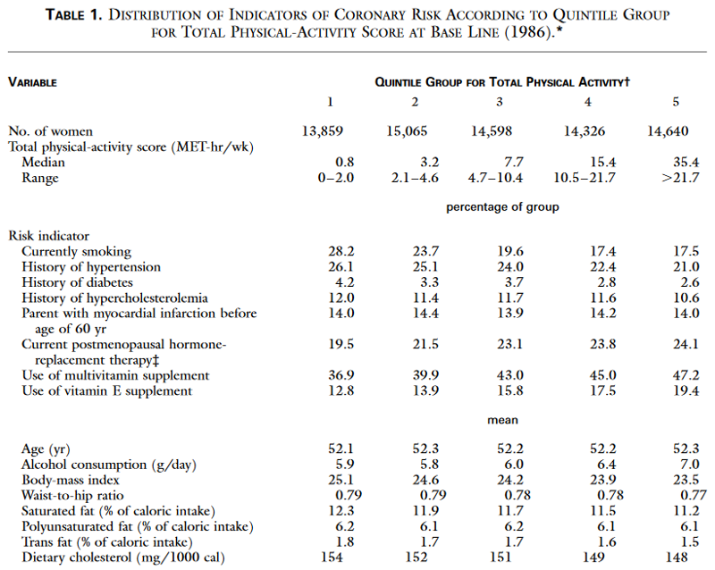
There are columns for each of the five quintiles in order from the least active to the most active. The rows list many variables that characterize the subjects and could also be confounders. Note that dichotomous variables are listed first and the percent with a given characteristic is listed for each quintile. For example, 28.2% of quintile 1 were current smokers, and this decreased steadily to 17.5% in the most active group (quintile 5). Therefore, smoking will be a potential confounding factor, because it is a risk factor for cardiovascular disease, and it differs among the exposure groups. Other possible confounding factors in table 1 include history of hypertension, history of diabetes, history of hypercholesterolemia (high blood levels of cholesterol), current use of hormone replacement therapy, use of multivitamins, and use of vitamin E supplements.
Continuous variables are listed in the lower half of Table 1, showing the mean value for each quintile of activity. Age is a risk factor for cardiovascular disease, but it is unlikely to cause confounding in this particular study, because the mean age is 52.1-52.3 years in all five quintiles. However, some of the other continuous variables do differ across the exposure groups, e.g., body mass index, alcohol consumption, and dietary cholesterol. Overall, increasing activity seems to be associated with trends in characteristics associated with a healthier lifestyle. If our goal is to understand the independent effect of exercise on risk of heart disease, then one must adjust for as many of these confounding factors as possible in the subsequent analysis. You will learn how to do this later in the course when we discuss confounding more completely.
You learned how to use R to generate descriptive statistics in the introductory module on R, and you have the tools to generate a table like Manson's Table 1 from a data set. The only other tool that you need is how to generate descriptive statistics in subsets of the data, e.g., the quintiles in the study by Manson et al. Methods for sub-setting are presented on the next page.