


Incidence
In contrast to prevalence, the numerator for incidence is the number of new cases of disease that develop during a period of observation, i.e., incidence focuses on the transition from non-diseased to diseased among those who are "at risk" of developing the disease. Therefore, for incidence calculations the denominator only includes people in the source population who were at risk of developing the outcome of interest at the beginning of the observation period. For an incidence calculation we exclude those who already have the outcome of interest or are not at risk of developing it.
The table below provides some clarifying examples.
|
Outcome of Interest |
Who to Exclude |
|---|---|
|
1st heart attack in adults |
Those who already had a heart attack |
|
Any heart attack in adults |
None (You need to consider the outcome of interest to decide who to exclude.) |
|
Polio in Pakistan |
Those who have received polio vaccine or who have had polio |
|
Cancer of the uterus |
Exclude men and any women who have had a hysterectomy.or who have already had uterine cancer |
Cumulative Incidence Versus Incidence Rate
There are two ways of measuring incidence: cumulative incidence and incidence rate. They are similar in that the numerator for both is the number of new cases that developed over a period of observation.
They are different in how they express the dimension of time.
- Cumulative incidence is the proportion of people who develop the outcome of interest during a specified block of time.
- Incidence rate is a true rate whose denominator is the total of the group's individual times "at risk" (person-time).
Cumulative Incidence
Cumulative incidence is the proportion of a population at risk that develops the outcome of interest over a specified time period .


The relevant time period must be stated in words.
Note: Cumulative incidence does not take into account :
- People who became lost to follow up during the observation period.
- When people developed the outcome.
Consider the time line below showing events in a hypothetical class that took place from January to May 2018. The instructor wanted to measure the cumulative incidence of upper respiratory tract infections (cold and flu) during the semester among the 80 students who enrolled in the class in January. The outcome was defined as the development of the first episode of cold or flu-like symptoms in a given student during the semester. The timeline shows that 20 students developed this outcome at varying times during the semester. In addition, five students dropped out of the course during the first two months. None of these "drops" had developed symptoms prior to leaving, but we have no way of knowing whether they developed a cold or flu after dropping out.
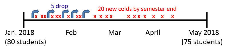
In this scenario:

This represents the proportion of the class that developed the outcome during a fixed block of time, and the time period is described in words. "The cumulative incidence was 25% during spring semester of 2018."
Several things are noteworthy:
- The cumulative incidence does not take into account drop outs (loss to follow-up); the denominator is the number of students enrolled in at the beginning in January.
- Students are no longer "at risk" of developing their first cold of the semester once they develop a cold, but cumulative incidence does not take into account their "time at risk" i.e., when they got the cold or when they dropped out.
- Cumulative incidence is a proportion that provides an estimate of the risk (i.e., probability) of developing disease, not the rate.
 Test Yourself
Now reconsider the previous hypothetical example on lung cancer in a population of 1,000 followed from 2001 to 2012. Recall that among the 1,000 subjects, 990 remained alive and free of cancer from 2001 to 2012. Subjects 1, 2, 3, and 4 were known to have lung cancer in 2001, and six new cases occurred from 2001 to 2012. The beginning of a dashed line indicates a newly diagnosed lung cancer, and the dashed lines indicate the ongoing presence of lung cancer in living subjects.
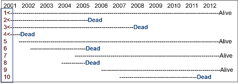
What was the cumulative incidence of lung cancer from 2001 to 2012? Compute your answer before looking at the correct answer.
It was noted above that cumulative incidence does not take into account time at risk, i.e., the specific when the health outcome occurred. To illustrate, consider the hypothetical comparison in the figure below, which compares two groups of ten people each. All 20 subjects had moderately severe knee pain from osteoarthritis. The first group received drug A and the second received drug B, and both groups were followed for ten hours. Every hour the subjects were asked if their pain had been substantially relieved, and the time at which they responded "yes" is marked with an "X".
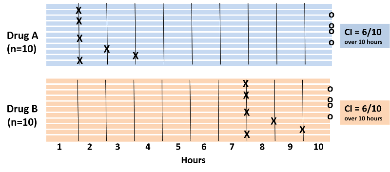
Note also that four subjects in each group did not experience pain relief during the ten hour period. With drug A six patients got pain relief in 1 to 3 hours. With drug B six patients reported pain relief after 7 to 9 hours. The cumulative incidence of pain relief is 6/10 over the ten hour observation period in both groups, but it is clear that the rate of pain relief is much faster with Drug A. The problem is that the cumulative incidence does not take into account when events of interest occured; it only measures the overall probability of occurrence. This limitation can be overcome if one records the time at which events occur and uses this to compute an incidence rate.
Incidence Rate
An incidence rate can be calculated only when there is ongoing follow-up of subjects who are at risk at the beginning of an observation period. By knowing when events of interest occur and approximately when losses to follow up occur, one can calculate each individual's "time at risk." The time at risk for each subject is the time from the beginning of their observation until one of three things occurs:
- An individual develops the outcome of interest (thus becoming no longer "at risk")
- An individual becomes lost to follow up or dies. If this occurs, we count the time that they were observed to be disease-free, but they stop contributing "time at risk" once they are lost to follow up or dead.
- The study ends.
One then adds up the total "time at risk" among all persons in the group (i.e., total person-time ) and uses this as the denominator in much the same way that one uses time to compute the flow rate of water. Therefore, person-time takes into account the number of people in the group and their time at risk.
The figure below depicts twelve subjects in a cohort study conducted over 14 years when the study ended. None of them had the outcome of interest at the beginning of the study, and all of them were enrolled in 1980. All subjects were contacted at two-year intervals and none of these subjects developed the health outcome of interest at any time during the study, and none were lost to follow-up. Therefore, each of the twelve subjects contributed 14 years of disease-free observation time during which they were "at risk." In this hypothetical mini-sample the concept of "person-time" is simple; the total person-time for the group is 168 years, because there were 12 subjects, and each of them was followed completely for 14 years without developing the outcome of interest. The total of 168 person-years represents 12 subjects who each contributed 14 years of disease-free time at risk.

One can also think about person-time in terms of the eligibility criteria for a study population. Individuals only contribute information while they are members of the source population and meet the eligibility criteria, two of which are that they are at risk of developing the outcome of interest and they are being followed, i.e., still active members of the group. With incidence rates, we conceptualize populations as the sum of observation times during which individuals meet the eligibility criteria. Each person contributes a specific amount of "person-time" to the overall experience of the population, so we can calculate a true rate.
Consider another group consisting of 12 people depicted below. None of the subjects had the disease of interest at the beginning of the study. Some subjects were enrolled in 1980 and others in were enrolled in 1981, and during the observation period, subjects 2, 5, and 11 developed the disease of interest after 10, 4, and 7 years of observation respectively. In addition, six subjects became lost to follow-up at various times, and only two subjects (#3 and #4) remained disease free all the way to 1994 when the study ended.
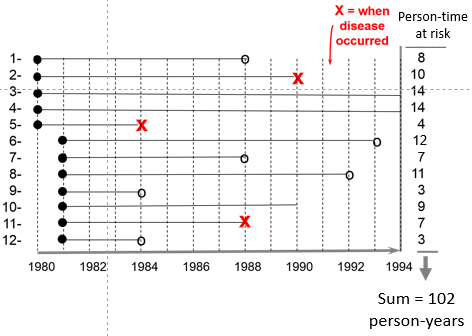
The sum of the years "at risk" of these 12 subjects is 102 person-years, and there were 3 occurrences of disease. We can now compute the incidence rate:

In this example,

Time is an inherent part of the calculated incidence rate, but one should still state the time period over which it was calculated, e.g., "The incidence rate was 2.9 per 100 person-years from 1980 to 1994."
Example:
The Black Women's Health Study followed 30,330 women for development of hypertension from 1997 to 2001. None of the subjects in this portion of the study had hypertension at the beginning of the observation period, but 2,314 had developed hypertension by 2001. The women who were studied contributed 104,574 person-years of hypertension-free observation time.

Interpretation: The incidence rate of developing hypertension in the Black Women's Health Study was 2,215 cases per 100,000 person-years from 1997 to 2001.
One can also think about person-time in terms of the eligibility criteria for a study population. Individuals only contribute information while they are members of the source population and meet the eligibility criteria, two of which are that they are at risk of developing the outcome of interest and they are being followed, i.e., still active members of the group. With incidence rates, we conceptualize populations as the sum of observation times during which individuals meet the eligibility criteria. Each person contributes a specific amount of "person-time" to the overall experience of the population, so we can calculate a true rate.
Incidence Density
Incidence rate is sometimes referred to as incidence density. Consider the hypothetical comparison of the incidence rate of heart attacks in the two hypothetical groups of subjects summarized by the illustration below which shows time on the horizontal axis and the number of subjects "at risk" on the vertical axis. The upper group consisted of non-exercisers and the lower group were exercisers. The "X"s indicate the new occurrence of a heart attack, and the white circles and black arrows indicate subjects who became lost to follow-up.
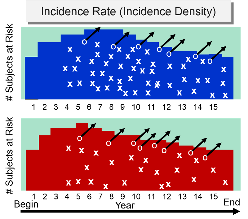
At the beginning of the study subjects without cardiovascular disease were enrolled into the study over a period of five years, so the number of subjects at risk increases in both groups increased during the first five years. After five years, the number of subjects at risk dwindled in both groups for three reasons: 1) enrollment of new subjects has ceased, 2) subjects in both groups began to develop heart disease, and 3) some subjects were lost to follow-up. The colored area under the graph depicts the total time at risk for each group, and all the "X"s represent the heart attacks that have occurred over the 15 year observation period. Note that the density of "X"s is greater in the non-exercisers, reflecting their greater incidence rate compared to the exercisers,
Which to Use: Cumulative Incidence or Incidence Rate?
Cumulative incidence and incidence rate are both useful, depending on the circumstance. The table below summarizes their appropriate use and their strengths
| Cumulative Incidence |
Incidence Rate |
|
|
Strengths |
|
|
|
Limitations |
|
|
|
Appropriate Use |
|
|
Summary of Measures of Disease Frequency
|
|


|
Prevalence - Probability of Current Disease |
Cumulative Incidence - Probability of New Disease (Risk) |
Incidence Rate Rate of New Disease - (Rate) |
|
|
Type |
Proportion |
Proportion |
Rate |
|
Range |
0-1 (or 0-100%) |
0-1 (or 0-100%) |
0 - ∞ |
|
Numerator |
Existing cases |
New cases |
New cases |
|
Denominator |
Total population |
Pop. at risk |
Person-time at risk |
|
Specify time? |
Yes |
Yes |
Yes |
|
Population |
Fixed or Dynamic |
Fixed (few lost) |
Fixed or Dynamic |
|
Uses |
Burden of disease |
Causes, impact of interventions |
Causes, impact of interventions |
Units for Denominators
By convention, all three measures of disease frequency (prevalence, cumulative incidence, and incidence rate) are expressed as some multiple of 10 in order to facilitate comparisons. Consider these three examples:
- Prevalence of HIV in US in 2003 = 8,263/5.7 million = 0.00145 = 145 per 100,000 persons in 2003
- Cumulative incidence: 4/10 over 6 years = 0.40 = 40 per 100 or 40% over 6 years
- Incidence rate: 3/107.7 person-yrs. = 0.02785 per person-year = 28 per 1,000 person-years
One can express the final result as the number of cases per 100 people, or per 1,000, or per 10,000, or per 100,000. Use a convenient multiple of 10 so that you can envision a whole number of people for comparison. For example, suppose we were comparing the incidence rate of a disease in Rhode Island and Massachusetts, and the incidence rate in Rhode Island is 0.00232 per person-year, while the incidence rate in Massachusetts is 0.00112 per person-year. It makes more sense to express these rates as 23.2 new cases per 10,000 person-years compared to 11.2 per 10,000 person-years, because we can think of this as two populations of 10,000 followed for a year with 23 new cases in the first and 11 new cases in the second. The expressions below are equivalent, but the last two expressions make it easier to envision whole people and make it easier to compare groups.
Note that each time you move the decimal to the right, you increase the base population by a factor of 10 as illustrated in the table below.
| Equivalent Expressions of Disease Frequency |
|---|
| 0.00232 new cases per 1 person-years |
| 0.0232 new cases per 10 person-years |
| 0.232 new cases per 100 person-years |
| 2.32 new cases per 1,000 person-years |
| 23.2 new cases per 10,000 person-years |
| 232 new cases per 100,000 person-years |

Common Pitfall: A common mistake among beginning students is to fail to specify the dimensions after calculating incidence, especially for cumulative incidence,
Here are examples of the correct way to express incidence:
- For cumulative incidence: "The cumulative incidence was 25% during the spring semester of 2018."
- For an incidence rate: "'The incidence rate was 2.9 per 100 person-years from 1980 to 1994."
Note: You must specify the time period for incidence calculations.
Test Yourself
Consider a group of 1,000 newborn infants. 100 infants were born with serious birth defects and 20 of these 100 died during the first year of life as a result of their birth defect. 90 of the 900 remaining infants without any birth defects also died during the first year of life. What is the overall cumulative incidence of mortality due to birth defects in this population? Compute this yourself before looking at the answer below.