PH717 - Module 3 - Measuring Frequency and Association

• Part 1 - Measures of Disease Frequency
• Part 2 - Measuring Association Between Exposures & Health Outcomes

Introduction

For centuries, knowledge about the cause of disease and how to treat or prevent it was limited because it was based mostly on anecdotal evidence. Significant advances occurred when the strategy for studying disease shifted to looking at groups of people and using a numeric approach to make critical comparisons.

Link to video transcript in a Word file

 Key Questions:

How do we measure the frequency of health outcomes?
How can I estimate the burden of disease in a population?
How do we design studies to determine whether an exposure is associated (linked) to a disease?
How can I estimate the risk of developing an adverse health outcome?
How do we detect associations?
How can I present basic information about exposure and outcome from a sample?

Learning Objectives

Part 1 - Measures of Disease Frequency

After successfully completing this section, you will be able to:

• Define, calculate and interpret measures of disease frequency: prevalence, risk (cumulative incidence) and incidence rate
• Explain the interrelationship among prevalence, incidence, and average duration of disease (i.e. P = IR x D). Be able to calculate the average duration of disease, given the prevalence and incidence rate.
• Calculate measures of frequency from raw data
• Explain what is meant by "person-time" and be able to calculate person-time and incidence rates

Part 2 - Measuring Association Between Exposures & Health Outcomes

After completing this section, you will be able to:

• Explain the design strategies and data obtained from prospective and retrospective cohort studies, intervention studies (clinical trials), and case-control studies
• Organize data from retrospective cohort studies, intervention studies (clinical trials), and case-control studies into a "2x2" contingency table
• Define and calculate prevalence ratio and prevalence difference; risk ratio and risk difference; rate ratio and rate difference
• Explain absolute and relative measures of association in words to scientific and lay audiences

Part 1 - Measures of Disease Frequency

Counting Cases of Disease

In order to estimate the frequency of a particular disease, we need to know:

• The number of cases of disease (the numerator)
• The size of the source population
• The relevant time period

The expression "frequency of disease" should be interpreted broadly to include any health outcome of interest (e.g., diseases, congenital defects, injuries, deaths, mental health problems)

There are many potential ways to collect information on health outcomes in a population:

• Medical records and reports of diagnostic tests
• Health insurance data bases
• Surveillance data from local, state, or federal health data bases
• Disease registries
• Death certificates
• Self-reports

A well-defined case definition ((i.e., criteria defining an individual with the health outcome of interest) is important for surveillance, investigation of acute disease outbreaks, and research on chronic diseases. Ill-defined definitions of outcomes can introduce errors in classification of health outcome status that can bias the results of these studies, (We will address misclassification bias later in the course).

Simple Ratios, Proportions, and Rates

Simple Ratios

A simple ratio is just a number that indicates the relative size of one measurement to another without implying any relationship between the numerator and the denominator. For example, if there were 100 women in a class and 20 men, the ratio of women to men would be 100/20 or 5 women for each man. This is just a simple ratio that indicates how many times larger one quantity is compared to the other.

Proportions

A proportion is a type of ratio that relates a part to a whole; expressed either as a fraction (e.g., 0.92) or as a percentage (e.g., 92%). For example, if there are 120 women in a class of 130 students, then the proportion of women is 120/130 = 0.92 = 92%.

Rates

A rate is a type of ratio in which the denominator also takes into account time. For example, speed is measured in miles per hour; it can be calculated by dividing the number of miles traveled by the number of hours that it took. Water flow can be quantified in gallons per minute; one might measure the number of gallons released during a period of time and divide by the number of minutes it took in order to calculate the average rate. An example of a rate that does not involve time is motor vehicle deaths, which are often reported as deaths per vehicle-miles traveled. This is one way in which the relative safety of different types of transportation (automobiles, buses, trains, airplanes) can be compared.

The term "rate" is used very broadly among the general population (birth malformation rate, autopsy rate, smoking rate, smoking rate, tax rate), but in reality all these measures are proportions. For example, the smoking "rate" among adults is actually the number of adults in a population who smoke divided by the total number of adults in the population, i.e., a proportion, because the numerator is a subset of the whole. One way to tell a proportion from a true rate is that a rate can never be expressed as a percentage, while a proportion can be expressed as a percentage.

Measures of Disease Frequency

 There are three fundamental measures of disease frequency:

1. Prevalence (the proportion of a population or group that has a specified condition)
2. Cumulative Incidence (the proportion of a population or group at risk that develops a new occurrence of a health outcome over a specified interval of time
3. Incidence Rate (the rate at which new cases of disease are occurring in a poulation at risk)

All three of these basic measures of disease frequency take into account:

• Definition of the population of interest (the eligibility criteria)
• The number of cases (the numerator)
• The size of the source population:
  • For prevalence the source population includes all people living in the population at the point in time when the cases are counted
  • For incidence the source population includes all people at risk of developing the health outcomes of interest at the beginning of the observation period
• The specified time during which outcomes were being counted

Prevalence

Prevalence is the proportion of a population that has the disease or condition of interest at a specified point in time, and it indicates the probability that a member of the population has a given condition at a point in time. It is, therefore, a way of assessing the overall burden of disease in the population at a given point in time. As such, it is a useful measure for administrators when assessing the need for services or treatment facilities. One way to think about prevalence is that it provides a "snapshot" of the proportion of the population with a specific condition at a point in time.

Prevalence is calculated as the number of people in a population who have a given disease at a specific point in time divided by the total number of people living in the population at that point in time.

 And the relevant time is stated in words.

 Example:

In 2003 it was estimated that there were 8,263 HIV+ people in Massachusetts. The population of MA in 2003 was about 5.7 million.

Note that the "total source population" does not always mean the total population; it means the total population of people in whom we are measuring prevalence. For example, the source population may consist of only females living in the population at that point in time.

Occasionally you will see the term period prevalence, which is similar to point prevalence, except that the "point in time" is broader.

Example:

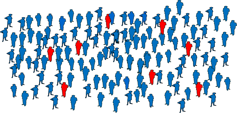
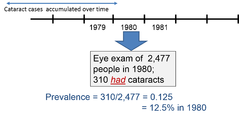
In 1980 the investigators in the Framingham Heart Study (FHS) wanted to determine the prevalence of cataracts in their current subjects. Some subjects had died since the beginning of the study in 1948, and some others had developed cataracts both before and since the start of the study. The investigators asked subjects to come to the FHS building to be examined for cataracts. During 1980, 2,477 subjects were examined, and 310 were found to have cataracts at that time. Therefore, the prevalence of cataracts was 310/2477= 0.125 = 12.5% in 1980.

Test Yourself

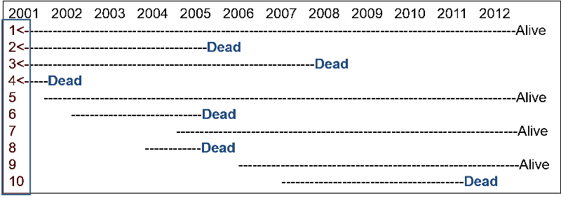
Consider a source population consisting of 1,000 adults. Assume that no subjects moved in or out of the population over the next 12 years, but there were some deaths. Among the 1,000 subjects, 990 remained alive and free of cancer from 2001 to 2012. Events in the other 10 subjects are depicted in the image below. Subjects 1, 2, 3, and 4 were known to have lung cancer in 2001. Dashed lines indicate the ongoing presence of lung cancer in living subjects (dashed lines), and deaths are indicated in the figure.

For this exercise answer the questions below as simple fractions showing the numerator and the denominator in order to make sure you understand prevalence. (Ordinarily, you would compute the decimal fraction and express in as, e.g., 7 per 1,000 population in 2007). Compute your own answers before looking at the correct answer.

Question 1: What was the prevalence of lung cancer in 2001?

Answer

Question 2: What was the prevalence of lung cancer in 2007?

 Answer

Question 3: What was the prevalence of lung cancer in 2012?

 Answer

Incidence

In contrast to prevalence, the numerator for incidence is the number of new cases of disease that develop during a period of observation, i.e., incidence focuses on the transition from non-diseased to diseased among those who are "at risk" of developing the disease. Therefore, for incidence calculations the denominator only includes people in the source population who were at risk of developing the outcome of interest at the beginning of the observation period. For an incidence calculation we exclude those who already have the outcome of interest or are not at risk of developing it.

The table below provides some clarifying examples.

Cumulative Incidence Versus Incidence Rate

There are two ways of measuring incidence: cumulative incidence and incidence rate. They are similar in that the numerator for both is the number of new cases that developed over a period of observation.

They are different in how they express the dimension of time.

• Cumulative incidence is the proportion of people who develop the outcome of interest during a specified block of time.
• Incidence rate is a true rate whose denominator is the total of the group's individual times "at risk" (person-time).

Cumulative Incidence

Cumulative incidence is the proportion of a population at risk that develops the outcome of interest over a specified time period .

The relevant time period must   be stated in words.

Note: Cumulative incidence does not take into account :

1. People who became lost to follow up during the observation period.
2. When people developed the outcome.

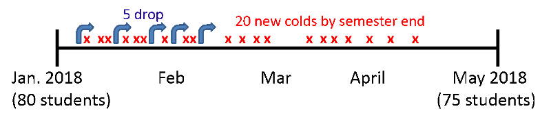
Consider the time line below showing events in a hypothetical class that took place from January to May 2018. The instructor wanted to measure the cumulative incidence of upper respiratory tract infections (cold and flu) during the semester among the 80 students who enrolled in the class in January. The outcome was defined as the development of the first episode of cold or flu-like symptoms in a given student during the semester. The timeline shows that 20 students developed this outcome at varying times during the semester. In addition, five students dropped out of the course during the first two months. None of these "drops" had developed symptoms prior to leaving, but we have no way of knowing whether they developed a cold or flu after dropping out.

In this scenario:

This represents the proportion of the class that developed the outcome during a fixed block of time, and the time period is described in words. "The cumulative incidence was 25% during spring semester of 2018."

Several things are noteworthy:

1. The cumulative incidence does not take into account drop outs (loss to follow-up); the denominator is the number of students enrolled in at the beginning in January.
2. Students are no longer "at risk" of developing their first cold of the semester once they develop a cold, but cumulative incidence does not take into account their "time at risk" i.e., when they got the cold or when they dropped out.
3. Cumulative incidence is a proportion that provides an estimate of the risk (i.e., probability) of developing disease, not the rate.

Test Yourself

Now reconsider the previous hypothetical example on lung cancer in a population of 1,000 followed from 2001 to 2012. Recall that among the 1,000 subjects, 990 remained alive and free of cancer from 2001 to 2012. Subjects 1, 2, 3, and 4 were known to have lung cancer in 2001, and six new cases occurred from 2001 to 2012. The beginning of a dashed line indicates a newly diagnosed lung cancer, and the dashed lines indicate the ongoing presence of lung cancer in living subjects.

What was the cumulative incidence of lung cancer from 2001 to 2012? Compute your answer before looking at the correct answer.

Answer

It was noted above that cumulative incidence does not take into account time at risk, i.e., the specific when the health outcome occurred. To illustrate, consider the hypothetical comparison in the figure below, which compares two groups of ten people each. All 20 subjects had moderately severe knee pain from osteoarthritis. The first group received drug A and the second received drug B, and both groups were followed for ten hours. Every hour the subjects were asked if their pain had been substantially relieved, and the time at which they responded "yes" is marked with an "X".

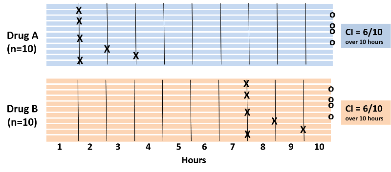
Note also that four subjects in each group did not experience pain relief during the ten hour period. With drug A six patients got pain relief in 1 to 3 hours. With drug B six patients reported pain relief after 7 to 9 hours. The cumulative incidence of pain relief is 6/10 over the ten hour observation period in both groups, but it is clear that the rate of pain relief is much faster with Drug A. The problem is that the cumulative incidence does not take into account when events of interest occured; it only measures the overall probability of occurrence. This limitation can be overcome if one records the time at which events occur and uses this to compute an incidence rate.

Incidence Rate

An incidence rate can be calculated only when there is ongoing follow-up of subjects who are at risk at the beginning of an observation period. By knowing when events of interest occur and approximately when losses to follow up occur, one can calculate each individual's "time at risk." The time at risk for each subject is the time from the beginning of their observation until one of three things occurs:

1. An individual develops the outcome of interest (thus becoming no longer "at risk")
2. An individual becomes lost to follow up or dies. If this occurs, we count the time that they were observed to be disease-free, but they stop contributing "time at risk" once they are lost to follow up or dead.
3. The study ends.

One then adds up the total "time at risk" among all persons in the group (i.e., total person-time ) and uses this as the denominator in much the same way that one uses time to compute the flow rate of water. Therefore, person-time takes into account the number of people in the group and their time at risk.

The figure below depicts twelve subjects in a cohort study conducted over 14 years when the study ended. None of them had the outcome of interest at the beginning of the study, and all of them were enrolled in 1980. All subjects were contacted at two-year intervals and none of these subjects developed the health outcome of interest at any time during the study, and none were lost to follow-up. Therefore, each of the twelve subjects contributed 14 years of disease-free observation time during which they were "at risk." In this hypothetical mini-sample the concept of "person-time" is simple; the total person-time for the group is 168 years, because there were 12 subjects, and each of them was followed completely for 14 years without developing the outcome of interest. The total of 168 person-years represents 12 subjects who each contributed 14 years of disease-free time at risk.

One can also think about person-time in terms of the eligibility criteria for a study population. Individuals only contribute information while they are members of the source population and meet the eligibility criteria, two of which are that they are at risk of developing the outcome of interest and they are being followed, i.e., still active members of the group. With incidence rates, we conceptualize populations as the sum of observation times during which individuals meet the eligibility criteria. Each person contributes a specific amount of "person-time" to the overall experience of the population, so we can calculate a true rate.

Consider another group consisting of 12 people depicted below. None of the subjects had the disease of interest at the beginning of the study. Some subjects were enrolled in 1980 and others in were enrolled in 1981, and during the observation period, subjects 2, 5, and 11 developed the disease of interest after 10, 4, and 7 years of observation respectively. In addition, six subjects became lost to follow-up at various times, and only two subjects (#3 and #4) remained disease free all the way to 1994 when the study ended.

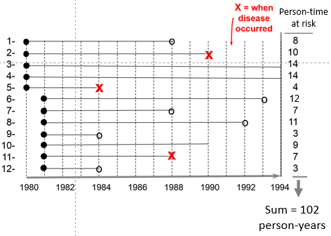
The sum of the years "at risk" of these 12 subjects is 102 person-years, and there were 3 occurrences of disease. We can now compute the incidence rate:

In this example,

Time is an inherent part of the calculated incidence rate, but one should still state the time period over which it was calculated, e.g., "The incidence rate was 2.9 per 100 person-years from 1980 to 1994."

Example:

The Black Women's Health Study followed 30,330 women for development of hypertension from 1997 to 2001. None of the subjects in this portion of the study had hypertension at the beginning of the observation period, but 2,314 had developed hypertension by 2001. The women who were studied contributed 104,574 person-years of hypertension-free observation time.

Interpretation:  The incidence rate of developing hypertension in the Black Women's Health Study was 2,215 cases per 100,000 person-years from 1997 to 2001.

One can also think about person-time in terms of the eligibility criteria for a study population. Individuals only contribute information while they are members of the source population and meet the eligibility criteria, two of which are that they are at risk of developing the outcome of interest and they are being followed, i.e., still active members of the group. With incidence rates, we conceptualize populations as the sum of observation times during which individuals meet the eligibility criteria. Each person contributes a specific amount of "person-time" to the overall experience of the population, so we can calculate a true rate.

Incidence Density

Incidence rate is sometimes referred to as incidence density. Consider the hypothetical comparison of the incidence rate of heart attacks in the two hypothetical groups of subjects summarized by the illustration below which shows time on the horizontal axis and the number of subjects "at risk" on the vertical axis. The upper group consisted of non-exercisers and the lower group were exercisers. The "X"s indicate the new occurrence of a heart attack, and the white circles and black arrows indicate subjects who became lost to follow-up.

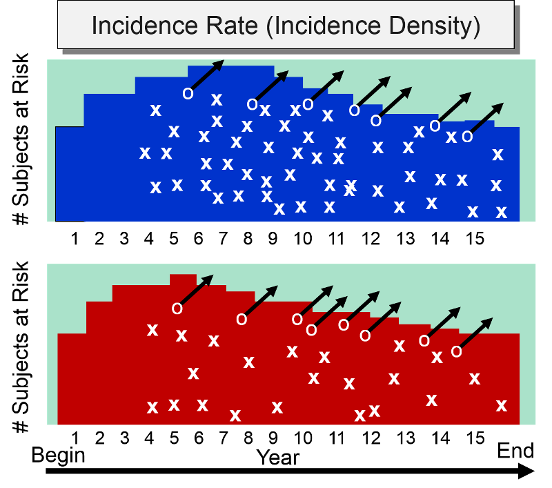
At the beginning of the study subjects without cardiovascular disease were enrolled into the study over a period of five years, so the number of subjects at risk increases in both groups increased during the first five years. After five years, the number of subjects at risk dwindled in both groups for three reasons: 1) enrollment of new subjects has ceased, 2) subjects in both groups began to develop heart disease, and 3) some subjects were lost to follow-up. The colored area under the graph depicts the total time at risk for each group, and all the "X"s represent the heart attacks that have occurred over the 15 year observation period. Note that the density of "X"s is greater in the non-exercisers, reflecting their greater incidence rate compared to the exercisers,

Which to Use: Cumulative Incidence or Incidence Rate?

Cumulative incidence and incidence rate are both useful, depending on the circumstance. The table below summarizes their appropriate use and their strengths

Summary of Measures of Disease Frequency

Units for Denominators

By convention, all three measures of disease frequency (prevalence, cumulative incidence, and incidence rate) are expressed as some multiple of 10 in order to facilitate comparisons. Consider these three examples:

• Prevalence of HIV in US in 2003 = 8,263/5.7 million = 0.00145 = 145 per 100,000 persons in 2003
• Cumulative incidence: 4/10 over 6 years = 0.40 = 40 per 100 or 40% over 6 years
• Incidence rate: 3/107.7 person-yrs. = 0.02785 per person-year = 28 per 1,000 person-years

One can express the final result as the number of cases per 100 people, or per 1,000, or per 10,000, or per 100,000. Use a convenient multiple of 10 so that you can envision a whole number of people for comparison. For example, suppose we were comparing the incidence rate of a disease in Rhode Island and Massachusetts, and the incidence rate in Rhode Island is 0.00232 per person-year, while the incidence rate in Massachusetts is 0.00112 per person-year. It makes more sense to express these rates as 23.2 new cases per 10,000 person-years compared to 11.2 per 10,000 person-years, because we can think of this as two populations of 10,000 followed for a year with 23 new cases in the first and 11 new cases in the second. The expressions below are equivalent, but the last two expressions make it easier to envision whole people and make it easier to compare groups.

Note that each time you move the decimal to the right, you increase the base population by a factor of 10 as illustrated in the table below.

Common Pitfall: A common mistake among beginning students is to fail to specify the dimensions after calculating incidence, especially for cumulative incidence,

Here are examples of the correct way to express incidence:

• For cumulative incidence: "The cumulative incidence was 25% during the spring semester of 2018."
• For an incidence rate: "'The incidence rate was 2.9 per 100 person-years from 1980 to 1994."

Note: You must specify the time period for incidence calculations.

Test Yourself

Consider a group of 1,000 newborn infants. 100 infants were born with serious birth defects and 20 of these 100 died during the first year of life as a result of their birth defect. 90 of the 900 remaining infants without any birth defects also died during the first year of life. What is the overall cumulative incidence of mortality due to birth defects in this population? Compute this yourself before looking at the answer below.

Answer

Relationship Among Prevalence, Incidence Rate, and Average Duration of Disease

Prevalence and incidence measure different phenomena, but they are related. Prevalence is the proportion of a population that has a condition at a specific time, but the prevalence will be influenced by both the rate at which new cases are occurring (incidence) and the average duration of the disease. Incidence reflects the rate at which new cases of disease are being added to the population (and becoming prevalent cases). Average duration of disease is also important, because the only way you can stop being a prevalent case is to be cured or to move out of the population or die. A prevalent case stops being a prevalent case if she is cured, and she also is no longer a prevalent case in the population if she dies or moves out of the population.

The relationship can be visualized by thinking of inflow and outflow from a sink.

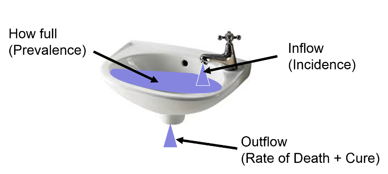
The fullness of the sink (as a percentage) can be thought of as analogous to prevalence, i.e., the proportion or percentage of the population with a given disease at a point in time. The rate at which water flows into the sink represents incidence or the rate at which new cases of a disease are being added to the population; think of each drop added to the sink as a new case. Once new cases are added to the population, they become prevalent cases. Water (i.e., prevalent cases) also can leave via the drain, which is analogous to removal of prevalent cases by virtue of either dying or being cured of the disease; each drop leaving the basin via the drain is no longer a prevalent case by virtue of either dying or being cured.

Now imagine that prevalence of a disease is relatively constant over time because the incidence (inflow from the faucet) and the rate of cure or death (outflow from the drain) are initially equal; if so, the height of water in the reservoir will remain constant.

• If outflow from the sink (rates of cure or death among prevalent cases) remains constant and inflow (incidence of new disease) increases, then the height of water in the reservoir will rise, meaning that prevalence has increased.
• If rates of death and/or cure are constant, and incidence declines, then the water level will fall, i.e. prevalence declines.

Now start from the steady state again.

• if the incidence of disease remains constant, but the rate of death from the disease or the rate of cure increases, then prevalence (fullness of the basin) will decline.
• If incidence remains constant, but the lives of prevalent cases are prolonged, but they aren't cured, then the prevalence will rise.

Example: HIV Prevalence in Kenya from 1990-2006

Prevalence is the proportion of the population with a specific disease at a point in time, but it can be measured at multiple points in time, i.e., serially, as shown in the figure below which displays the prevalence of HIV in Kenya, measured each year from 1990 to 2006.

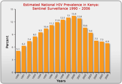
Source: http://www.avert.org/hiv-aids-kenya.htm

The steady increase in prevalence of HIV from 1990 to 2000 was primarily due to the availability of anti-retroviral drugs, which kept those infected with HIV from dying. The antiretrovirals did not cure them, however, so they remained prevalent cases for a longer period of time (i.e., the average duration of disease increased), and the prevalence increased. After the year 2000, the availability of antiretrovirals fell, and the mortality rate from AIDS began to climb again. As a result, the average duration of disease declined, and the prevalence fell.

Several decades ago the average duration of lung cancer was about six months. Therapy was ineffective and almost all lung cancer cases died. From the time of diagnosis, the average survival was only about six months. As a result, the prevalence of lung cancer was fairly low, because the average duration of disease was short. In contrast, diabetes has a long average duration, since it can't be cured, but it can be controlled with medications for many years, so the average duration of diabetes is long, and the prevalence is fairly high.

If the population is initially in a "steady state," meaning that prevalence is fairly constant and incidence and outflow [cure and death] are about equal), then the relationship among these three parameters can be described mathematically as:

Mathematical Relationship Among Prevalence, Incidence, and Average Duration of Disease

If the population is initially in a "steady state," meaning that prevalence is fairly constant and incidence and outflow [cure and death] are about equal), then the relationship among these three parameters can be described mathematically as:

where P= proportion of the population with the disease and (1-P) is the proportion without it, IR is the incidence rate, and "Average duration of disease" is the average time that people have the disease (from diagnosis until they are either cured or die). If the prevalence of disease is low (i.e., <10% of the population has it), then the relationship can be expressed as follows: 

• If the average duration of disease remains constant, then preventive measures that reduce the incidence of disease would be expected to result in a decreased prevalence.
• Similarly, if the incidence remained constant, then developing a cure would reduce the average duration of disease, and this would also reduce the prevalence of disease.

In the late 1990s anti-retroviral therapy was introduced and greatly improved the survival of people with HIV. However, they weren't cured of their disease, meaning that the average duration of disease increased. As a result, the prevalence of HIV increased during this period.

Calculating Average Duration of Disease

The relationship above can be used to calculate average duration of disease under steady state circumstances. If Prevalence = (Incidence) X (Average Duration), then:      

Example:

Suppose the incidence rate of lung cancer is 46 new cancers per 100,000 person-years, and the prevalence is 23 per 100,000 population. If so, then,

Individuals with lung cancer survived an average of 6 months from the time of diagnosis

Test Yourself

Special Measures of Disease Frequency

Special Measures of Incidence

Morbidity rate is the incidence of non-fatal cases of a disease in a population during a specified time period. For example, during 1982 there were 25,520 non-fatal cases of TB in the US population. The mid-year population was estimated at 231,534,000. Therefore,

Morbidity rate of TB =25,520/231,534,000  = 11.0/100,000 over one year 

Note that this is a cumulative incidence and therefore is really a proportion, not a true rate.)

Mortality Rate: In 1982 there were 1,807 deaths from TB in the US population, so the mortality rate for TB was 7.8 per million over one year (also a cumulative incidence, not a true rate).

Case-Fatality Rate: the number of deaths from a specific disease divided by the total number of cases of that disease, i.e. the proportion of fatal cases of a disease (%). This provides a measure of the severity of the disease.

Example: Reyes Syndrome is a rare, but highly fatal disease in which the liver and brain become dysfunctional due to abnormal accumulation of cellular fat. It tends to occur when people are recovering from a viral illness, and it tends to be associated with use of aspirin, especially in children. If there were 200 cases of Reyes syndrome in 1982 and 70 died, then the case-fatality rate would be 70/200 = 35% over one year. 

[Note: Case-fatality rates are generally calculated by dividing the deaths reported in a given year by the number of cases reported in the same year, but this can be misleading since some diseases (e.g., TB) aren't rapidly fatal. Thus, many of the TB fatalities that occurred in 1982 were due to cases diagnosed several years earlier.]

Attack Rate: a cumulative incidence for a disease during a specific period (e.g., an epidemic).

Example: After a church picnic in Oswego, NY many attendees got food poisoning. There were 75 people at the picnic; 46 got sick within several hours, so the attack rate was 46/75 = 61%.

Live Birth Rate: the frequency of live births in one year per 1,000 females of childbearing age.

Infant Mortality Rate: the frequency of deaths in children under 1 year of age occurring during a one year period per 1,000 live births.

Special Measures of Prevalence

These are often incorrectly referred to as incidences or rates, but they are, in fact, proportions..

Autopsy Rate: the proportion of people who have a particular finding on a postmortem exam (the prevalence of a certain finding among the population of people who get autopsied).

Birth Defect Rate: the prevalence of a congenital abnormality at the "point" of birth. The denominator can be either live births or total births (which includes live births + stillbirths), but it generally does not include spontaneously aborted fetuses.  

Part 2 - Measures of Association Between Exposure and Disease

When searching for the determinants of a health outcome, one generally relies first on descriptive epidemiology to generate hypotheses about associations between health-related exposures and outcomes. Once hypotheses are generated, analytical epidemiology is employed to  test hypotheses by drawing samples of people and comparing groups to determine whether health outcomes differ based on exposure status. If individuals with a given exposure are found to have a greater probability of developing a particular outcome, it suggests an association, and, conversely, if the groups have the same probability of developing the outcome regardless of their exposure status, it suggests that particular exposure is not associated with a greater risk of disease. In either event one must then consider whether the findings were misleading because of sampling error, bias, or confounding (the issue of validity is one that we will address later), In other words, we must consider alternative explanations that might invalidate our conclusions. The remainder of this module we will focus on methods for comparing groups and computing an estimate of the magnitude of association between an exposure and a health outcome and how to interpret the findings.

Basic Strategies for Analytical Epidemiology Studies

Study designs will be discussed more completely in a later module, but several basic design strategies are introduced here in order facilitate an understanding of how one measures the magnitude of an association.

Cross-sectional surveys were discussed in module 1B on descriptive studies. These studies assess exposure status and health outcome status at a single point in time, providing prevalence measures.

Cohort studies enroll a sample of subjects who do not yet have the health outcomes of interest and assess their exposure status, e.g., whether they smoke or not, and then follow the subjects forward in time and record whether they develop a particular health outcome, such as coronary heart disease. When sufficient time has passed, the subjects are grouped according to their exposure status, and the incidence of disease is compared among two or more levels of exposure. For example, a greater incidence of heart disease in smokers than in non-smokers suggests that smoking is associated with a greater risk of coronary heart disease. If the cohort study is conducted in a way that provides individual follow-up, it is possible to record when outcomes occur and if and when subjects become lost to follow-up. This then provides the option of computing either cumulative incidence or incidence rates. The basic design of a cohort study is illustrated in the figure below.

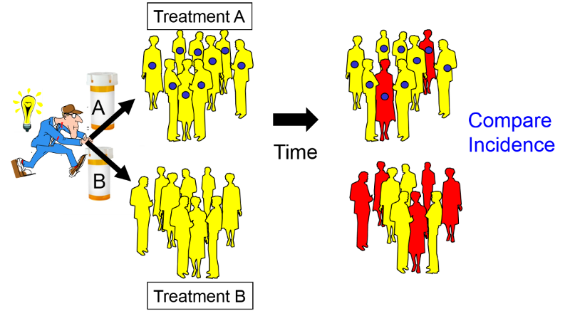
Intervention studies (randomized clinical trials) are similar in design to cohort studies in that they enroll subjects who do not yet have the outcome of interest, and subjects are followed over time in order to compare incidence of the outcome among two or more exposure groups. However, in contrast to cohort studies, exposures are allocated to subjects by the investigators, usually in a randomized fashion. For example, if investigators wanted to test the efficacy of low-dose aspirin (test agent A) in preventing heart attacks compared to an inactive placebo (test agent B), eligible subjects would be randomly allocated to take either agent A or agent B, as illustrated in the image below.

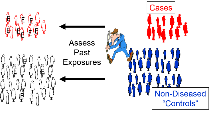
Case-control studies use a different analytic strategy. They enroll a group of "cases" who already have the outcome of interest, and then they enroll a comparison group of "controls" who do not. Investigators then assess past exposures in the two groups and compare the odds of past exposure. Greater odds of exposure in the cases suggests an association. Note that in the illustration below the odds of exposure (indicated by the letter "E") are greater among the case subjects than in the non-diseased control subjects.

We will address these design strategies in greater detail in subsequent modules, but for now we will focus on formulating hypotheses and then testing hypotheses by computing measures of association in cross-sectional surveys, cohort studies, and intervention studies.

Hypotheses

A hypothesis is a testable statement that tries to explain relationships, and it can be accepted or rejected through scientific research.

A fundamental hypothesis expresses one's belief or suspicion about a relationship, e.g., " Smoking causes lung cancer." This statement is not easily testable, however.

A research hypothesis is a more precise and testable statement, such as, " People who smoke cigarettes regularly will have a higher incidence of lung cancer over a 10-year period than people who do not smoke cigarettes."

The Null Hypothesis:

We test hypotheses by taking samples of people from a population, and there is always the possibility that the results will be misleading if the samples are not representative of the population from which they were drawn. This is called sampling error or random error, i.e., "the luck of the draw".

In order to assess the likelihood of sampling error, we reframe the research hypothesis as a null hypothesis , such as, " Over a 10-year period the incidence of lung cancer is the same in people who smoke regularly compared to those who do not. "

By beginning with the null hypothesis, one can quantify the magnitude of difference between the groups in the samples and ask, "What is the probability of seeing a difference in this great or greater due to sampling error?" In the probability that the difference was due to sampling error is very low, then we have sufficient evidence to reject the null hypothesis (i.e., conclude that it is probably not correct), leading us to accept the alternative hypothesis, i.e., that the groups are different. If the probability of sampling error is not low, we conclude that there is insufficient evidence to conclude that there is a difference. This does not mean that the groups are the same, however; it just means there was insufficient evidence to conclude that they differ.

Measures of Association Summarize Comparisons of Frequency

In cross-sectional surveys and cohort studies we can compute the frequency of disease in each exposure group, and we can compare them by either looking at their ratio (dividing one frequency by the other) or their difference (subtracting one frequency from the other).

• Depending on how detailed follow-up is, cohort studies provide the option of using either cumulative incidence in the exposed group (CI_e) and unexposed group (CI_u) or incidence rate in the exposed group (IR_e) and unexposed group (IR_u).
• Cross-sectional studies provide prevalence of exposure (P_e) and prevalence of outcome (P_u).

Ratios (relative measures)

• Risk Ratio: ratio of CI_e/CI_u
• Incidence Rate Ratio: IR_e/IR_u
• Prevalence Ratio: P_e/P_u

Differences (absolute measures)

• Risk Difference: CI_e - CI_u
• Rate Difference: IR_e - IR_u
• Prevalence Difference: P_e - P_u

Contingency Tables

Contingency tables make it easier to summarizes counts by exposure and outcome status.

One method lists outcome categories in the rows and the exposure categories in the column as shown in the table below. The letters "a", "b", "c", and "d" represent the number of subjects in each category.

 An alternate method lists outcome categories in columns and the exposure categories in rows as shown in the next table.

Either method is acceptable, but you should be consistent and be clear about which orientation is being used, because it will affect subsequent calculations.

Consider the following example illustrating a cohort of freshmen in high school who were enrolled in a cohort study in 1990. None of them had respiratory diseases at the time, but a number of them had begun smoking (indicated by the blue dots). When the cohort was re-examined in 2018, many of the subjects had developed respiratory disease, as shown by the red icons.

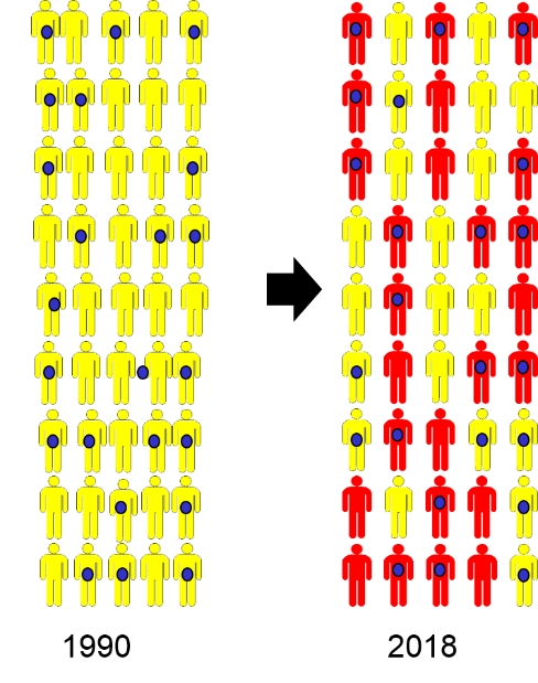
This information could be summarized with a contingency table as follows:

Alternatively, the data could be summarized with the other orientation:

In this example the tables summarize the counts for two exposure categories and two outcome categories, so they are often referred to as "2 x 2" tables ("2 by 2"). The exposed group is also referred to as the "index" group, and the unexposed group is referred to as the "reference" or "comparison" group.

It is also possible to have more than two categories of exposures or outcomes. For example,

Smoking

• Smoke >2 packs/day
• Smoke 1-2 packs/day
• Smoke <1 pack/day
• Never-smoker [This is the logical "reference" or "comparison" group.]

Amount of Exercise

• Highest quintile
• Quintile 4
• Quintile 3
• Quintile 2
• Lowest quintile [This is the logical "reference" or "comparison" group.]

BMI

• <20
• 20 – 24.9 [This is "normal" BMI & would be a logical reference group.]
• 25.0 – 29.9
• ≥ 30.0

In these examples the reference group is the group against which the other categories would be compared. However, note that sometimes selection of a reference group is arbitrary. For exercise, for example, we might have designated the highest quintile as the reference group and compared the other exposure groups to the most active group.

Risk Ratio and Risk Difference

In the example above comparing the incidence of respiratory disease in smokers and non-smokers, the cumulative incidence (risk) of respiratory disease in smokers was 9/10=0.90 (or 90%), while in non-smokers the cumulative incidence (risk) was 7/12=0.58 (or 58%). The ratio of these is the risk ratio, a relative measure of association.

Risk Ratio = CI_e/CI_u = 0.90/0.58 = 1.55

Interpretation: Smokers had 1.55 times the risk of respiratory disease compared to non-smokers over an 18 year period of observation.

Using the same cumulative incidences we can calculate the risk difference, an absolute measure of association.

Risk Difference = CI_e- CI_u = 0.90 - 0.58 = 0.32 = 32 per 100

Interpretation: Among smokers there were 32 excess cases of respiratory disease per 100 smokers during the 18 year study.

It is also possible for a risk ratio to be <1 if the exposure is associated with a reduction in risk. In 1982 The Physicians' Health Study (a randomized clinical trial) was begun to test whether low-dose aspirin reduced the risk of myocardial infarctions (heart attacks). The study population consisted of over 22,071 male physicians randomly assigned to either low-dose aspirin or a placebo (an identical looking pill that was inert). They followed these physicians for about five years. Some of the data is summarized in the 2x2 table shown below.

• With aspirin cumulative incidence = 139/11,037 = 0.0126 = 1.26%
• With placebo cumulative incidence = 239/11,034 = 0.0217 = 2.17%

Risk Ratio =  0.0126/0.0217 = 0.58

Note that the "exposure" of interest was low-dose aspirin, and the aspirin group is summarized in the top row. The group assigned to take aspirin had an incidence of 1.26%, while the placebo (unexposed) group had an incidence of about 2.17%. The cumulative incidence in the aspirin group was divided by the cumulative incidence in the placebo group, and RR= 0.58.

Interpretation: Male physicians who took 325 mg of aspirin every other day had 0.58 times the risk (i.e., a 42% reduction in risk) of myocardial infarction compared to those who received a placebo.

Risk Difference = 0.0126 – 0.0217 = - 0.0091 = - 91/10,000

Note that the index group (i.e., with the exposure of interest) always comes first when computing a measure of association. For a risk ratio the incidence in the group with the exposure of interest is in the numerator, and the incidence for the reference group is in the denominator. For a risk difference the incidence in the reference group is subtracted from the incidence in the group with the exposure of interest.

Also note that the risk difference in the aspirin study was a negative number, again indicating that taking aspirin was associated with a reduction in risk. Interpretation: Male physicians taking 325 mg of aspirin every other day had 91 fewer myocardial infarctions per 10,000 men during the five year study.

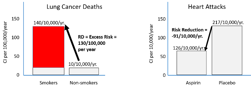
Harmful exposures create excess risk, and preventive measures reduce risk as shown in the figure below. The left side illustrates the excess risk of lung cancer deaths among smokers compared to non-smokers. The right side shows the reduction in risk of heart attack among men taking low-dose aspirin compared to men taking a placebo.

Excess Relative Risk

Suppose a study found that the cumulative incidence of coronary heart disease (CHD) was 3.2/1000 among subjects with hypertension and 1.2/1000 among those without hypertension.

The Risk Ratio = 2.7, and we could interpret this as:

Those with hypertension had 2.7 times the risk of CHD compared to those without hypertension during the study period.

If the risk were equal in the two groups the risk ratio would be 1, so we could also interpret this as an excess relative risk of 170%, i.e., the percent increase in risk compared to the baseline incidence in the reference group.

Those with hypertension had 2.7 times the risk, which is the same as a 170% increase in risk compared to those without hypertension during the study period.

Excess Relative Risk = (RR-1) x 100%

The "Null" Values

The null value is to the measure of association when the incidence is the same in the groups being compared. If this is the case, the risk ratio = 1, the risk difference = 0, and the excess relative risk = 0.

Incidence Rate Ratios and Incidence Rate Differences

For cohort studies with ongoing, periodic individual follow-up, we can determine the "time at risk," which enables us to compute and compare incidence rates.

We can summarize the findings with another contingency table with the general form shown in the table below. Again, "a", "b", "c", and "d" represent the number of subjects in each category, and P-Y_e and P-Y_u represent the total person-years of disease-free observation time in the exposed and unexposed subjects, respectively.

Incidence rate in the exposed group:     IR_e = a/ P-Y_e
Incidence rate in the unexposed group: IR_u = c/ P-Y_u

Consider the following example from the Nurses' Health Study which studied a large cohort of nurses for many years. The contingency table below summarizes data for a study looking at the association between body mass index (BMI) and development of a non-fatal myocardial infarction. No data is shown for subjects who did not have a myocardial infarction, because for each exposure group we only need the number who had an infarction and the total person-years of disease-free observation.

These data can be used to calculate incidence rates per 100,000 person-years, the incidence rate ratio, and the incidence rate difference per 100,000 person-years as shown in the table below.

See if you can replicate these calculations from the contingency table above.

If we compare the incidence rate in the heaviest to the leanest women:

Incidence rate ratio = IRR = (85.4/100,000 PY) / (23.1/100,000 PY) = 85.4/23.1 = 3.7

Interpretation: Women with BMI > 30 had 3.7 times the rate of having a non-fatal myocardial infarction compared to women with BMI < 20 during the study period.

And

Incidence rate difference = IRD = 85.4/100,000-23.1/100,000 = 62/100,000 PY

Interpretation: Among the heaviest women there were 62 excess cases of non-fatal MI per 100,000 person-years of follow-up that could be attributed to their excess weight during this study period.

This suggests, for example, that if we followed another 50,000 women with BMI > 30 for 2 years we might expect 62 excess non-fatal myocardial infarctions due to their weight(since 50,000 persons with complete follow-up for 2 years would provide 100,000 person-years of follow-up). Or one could prevent 62 non-fatal myocardial infarctions by getting them to reduce their weight.

Prevalence Ratio & Prevalence Difference

Suppose we had data from a cross-sectional survey that had asked whether people currently smoked and whether they currently had problems with wheezing and coughing. You could use a 2x2 table to organize the data from the 100 respondents as in the table below:

• Prevalence of wheezing and coughing among smokers = 13/26=0.50.
• Prevalence of wheezing and coughing among non-smokers = 2/74=0.027.

Prevalence Ratio = PR = 0.50/0.027 = 18

Interpretation: Smokers had 18 times the prevalence of wheezing and coughing compared to non-smokers.

Prevalence Difference = PD = 0.5-0.027=0.473 = 47.3 per 100

Interpretation: Among smokers there were 47 excess cases of wheezing and coughing per 100 compared to non-smokers in a given time period.

Based on this cross-sectional data, I might hypothesize an association between smoking and respiratory problems, but the temporal relationship is unclear, and an analytical study would be a good next step.

Absolute and Relative Measures Provide Different Perspectives

Absolute measures of association, such as risk differences and incidence rate differences, like risk difference and incidence rate difference quantify excess risk or rate of disease in the exposed group compared to the unexposed group, and this provides a measure of the actual number of people who might be affected and the potential public health impact of the exposure, providing a focus on two key questions:

• How much impact would prevention have?
• How many people would benefit?

Relative measures of association, such as risk ratio and rate ratio quantify the relative risk or rate of disease in an exposed group compared to an unexposed group and tend to be thought of as representing the strength of the association between an exposure and a disease by addressing questions such as:

• How much more likely are exposed persons to develop the outcome than the unexposed?

To illustrate consider the annual cumulative incidence death from lung cancer and the annual cumulative incidence of death from heart disease in smokers and non-smokers.

Mortality Rate from Lung Cancer

• Smokers: 140/100,000 per year
• Non-smokers: 10/100,000 per year

Risk ratio = 140/10 = 14
This suggests that smokers have 14 times the risk of dying of lung cancer compared to non-smokers over a year.
Risk difference = 140/100,000 – 10/100,000 = 130/100,000 per year
The same data suggests that if we had prevented 100,000 people from smoking, we would have prevented 130 lung cancer deaths per year.

Mortality rate from Heart Disease

• Smokers: 669/100,000 per year
• Non-smokers: 413/100,000 per year

Risk ratio = 669/413 = 1.6
This suggests that smokers have 1.6 times the risk of dying of lung cancer compared to non-smokers over a year.
Risk difference = 669/100,000 – 413/100,000 = 256/100,000 per year
This suggests that if we had prevented 100,000 people from smoking, we would have prevented 256 deaths from heart disease per year.

A bar chart summarizing these measures of association looks like this:

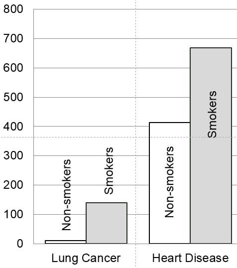
The bar chart emphasizes that the mortality rate from lung cancer is very low, but smoking is a very strong risk factor since it increases the risk 14-fold. In contrast, mortality from heart disease is more common even among non-smokers. The risk ratio for smoking and death from heart disease is only 1.6, or 60% greater in smokers than in non-smokers, but the risk difference is much greater for heart disease mortality than for lung cancer mortality, because heart disease is much more common. As a result, if we were to eliminate smoking, we would prevent more deaths from heart disease than from lung cancer. So, smoking is a stronger risk factor for lung cancer, but smoking causes more deaths from heart disease.

Relative measures of association are commonly used in journal articles presenting research findings on etiology, but absolute measures of association provide a better idea of public health impact, i.e., the number of people affected.

Using R to Generate Contingency Tables from a Data Set

So far you have been given the counts needed to summarize data in a contingency table, but what do you do if you don't have the counts and you have to get them from a large data set? Statistical packages like R make this simple. In order to illustrate, I created a subset of data from the Framingham Heart Study that I restricted to non-smokers with BMI > 20, and I called the file "fram-nosmoke-nolow.csv".

Our goal was to create a contingency table with three categories of exposure based on BMI (normal, overweight, or obese) and two categories of outcome based on the variable MI-FCHD (whether the subject had been hospitalized for a myocardial infarction or had died of coronary heart disease). MI-FCHD is coded 1 if true (occurred) and 0 if false. BMI is a continuously distributed variable in the data set, and I wanted to create a new variable with the three categories listed above using the "ifelse" function in R.

The "ifelse" function used below can be very useful. Here it is used to examine the continuous variable BMI and create a new variable called bmicat, which categorizes individuals based on BMI into one of three categories:

• "norm" (normal BMI: 20-25)
• "over" (overweight: BMI 25-29.99)
• "obese" (BMI >29.99)

The ifelse function uses the format:

ifelse(test_expression, x, y)

"test_expression" is a statement that can be evaluated as true or false. If it is true, "x" is used, and if false "y" is used.
In the code below I wanted to create a new variable called "bmicat" whose value was defined using a nested ifelse function:

> bmicat<-ifelse(BMI>29.99, "obese", ifelse(BMI>24.99, "over", "normal"))

This looks at the value of BMI in each record in the database; if BMI is greater than 29.99, it assigns a value of "obese" to bmicat and moves on to the next record. If BMI is not >29.9, it executes another ifelse function (i.e., nested), and if BMI>24.99 it assigns a value of "over" to bmicat and moves on to the next record. However, if BMI is not >24.99, it assigns a value or "normal" to bmicat.

The R code used to do thés is shown below. The statements that begin with the # symbol are comments embedded in the code that are ignored by R, i.e., not executed. Executed statements are shown below that in blue, and the resulting output is shown below that

# I imported fram-nosmoke-nolow.csv and nicknamed it "fr" # na.omit removes records that have missing values > fr<-na.omit(fram_nosmoke_nolow) > attach(fr) # The next command uses the ifelse command to create three categories of BMI
> bmicat<-ifelse(BMI>29.99, "obese", ifelse(BMI>24.99, "over", "normal"))
> table(bmicat,MI_FCHD)

(Output)
MI_FCHD
bmicat  0   1
norm  694  79
obese 296  50
over  800 123

# You can also generate the other format for the contingency table by switching the order of the variables
> table(M1_FCHD,bmicat)

(Output)

bmicat
M1_FCHD normal obese over
0    650   258 767
1     72    44  114

Note that MI-FCHD was coded I if it occurred and 0 if it did not. However, R defaults to listing the lower value first. It also defaults to listing the categories of bmicat in alphabetical order.

From this output I created the following contingency table:

We can also ask R for the proportion of "events" in each category of BMI as follows. Notice the use of a ",1" flag at the end of the command to get the row proportions.

prop.table(table(bmicat,MI_FCHD),1)

MI_FCHD
bmicat      0           1
normal 0.90027701 0.09972299
obese  0.85430464 0.14569536
over   0.87060159 0.12939841

Test Yourself

Using the contingency table above do the following before looking at the answers:

• Compute the cumulative incidence in obese subjects and those with normal BMI.
• Compute the risk ratio for obese compared to normal subjects.
• Interpret the risk ratio you calculated in a sentence.
• Compute the risk difference for obese compared to normal subjects.
• Interpret the risk difference you calculated in a sentence.

Answers