


The Normal Distribution: A Probability Model for a Continuous Outcome
Normal (Gaussian) Distributions
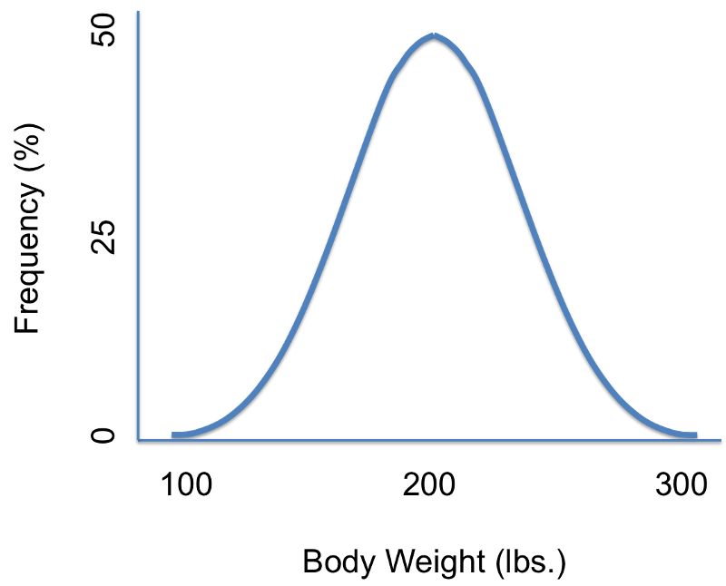
Suppose we were interested in characterizing the variability in body weights among adults in a population. We could measure each subject's weight and then summarize our findings with a graph that displays different body weights on the horizontal axis (the X-axis) and the frequency (% of subjects) of each weight on the vertical axis (the Y-axis) as shown in the illustration on the left. There are several noteworthy characteristics of this graph. It is bell-shaped with a single peak in the center, and it is symmetrical. If the distribution is perfectly symmetrical with a single peak in the center, then the mean value, the mode, and the median will be all be the same. Many variables have similar characteristics, which are characteristic of so-called normal or Gaussian distributions. Note that the horizontal or X-axis displays the scale of the characteristic being analyzed (in this case weight), while the height of the curve reflects the probability of observing each value. The fact that the curve is highest in the middle suggests that the middle values have higher probability or are more likely to occur, and the curve tails off above and below the middle suggesting that values at either extreme are much less likely to occur. There are different probability models for continuous outcomes, and the appropriate model depends on the distribution of the outcome of interest. The normal probability model applies when the distribution of the continuous outcome conforms reasonably well to a normal or Gaussian distribution, which resembles a bell shaped curve. Note normal probability model can be used even if the distribution of the continuous outcome is not perfectly symmetrical; it just has to be reasonably close to a normal or Gaussian distribution.
Skewed Distributions
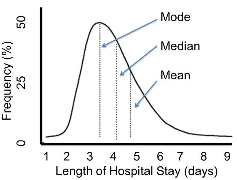
However, other distributions do not follow the symmetrical patterns shown above. For example, if we were to study hospital admissions and the number of days that admitted patients spend in the hospital, we would find that the distribution was not symmetrical, but skewed. Note that the distribution to the distribution below is not symmetrical, and the mean value is not the same as the mode or the median.
Characteristics of Normal Distributions
Distributions that are normal or Gaussian have the following characteristics:
- Approximately 68% of the values fall between the mean and one standard deviation (in either direction)
- Approximately 95% of the values fall between the mean and two standard deviations (in either direction)
- Approximately 99.9% of the values fall between the mean and three standard deviations (in either direction)
If we have a normally distributed variable and know the population mean (μ) and the standard deviation (σ), then we can compute the probability of particular values based on this equation for the normal probability model:
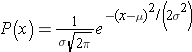
where μ is the population mean and σ is the population standard deviation. (π is a constant = 3.14159, and e is a constant = 2.71828.) Normal probabilities can be calculated using calculus or from an Excel spreadsheet (see the normal probability calculator further down the page. There are also very useful tables that list the probabilities.
BMI in Males
Consider body mass index (BMI) in a population of 60 year old males in whom BMI is normally distributed and has a mean value = 29 and a standard deviation = 6. The standard deviation gives us a measure of how spread out the observations are.
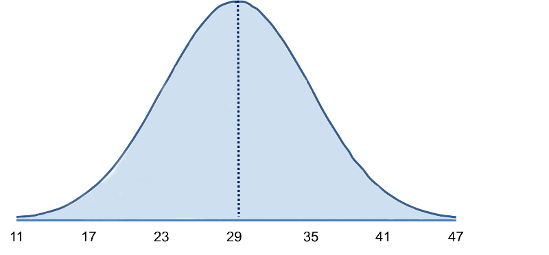
The mean (μ = 29) is in the center of the distribution, and the horizontal axis is scaled in increments of the standard deviation (σ = 6) and the distribution essentially ranges from μ - 3 σ to μ + 3σ. It is possible to have BMI values below 11 or above 47, but extreme values occur very infrequently. To compute probabilities from normal distributions, we will compute areas under the curve. For any probability distribution, the total area under the curve is 1. For the normal distribution, we know that the mean is equal to median, so half (50%) of the area under the curve is above the mean and half is below, so P(BMI < 29)=0.50. Consequently, if we select a man at random from this population and ask what is the probability his BMI is less than 29?, the answer is 0.50 or 50%, since 50% of the area under the curve is below the value BMI = 29. Note that with the normal distribution the probability of having any exact value is 0 because there is no area at an exact BMI value, so in this case, the probability that his BMI = 29 is 0, but the probability that his BMI is <29 or the probability that his BMI is < 29 is 50%.
What is the probability that a 60 year old male has BMI less than 35? The probability is displayed graphically and represented by the area under the curve to the left of the value 35 in the figure below.
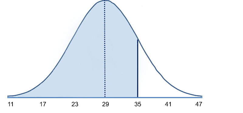
Note that BMI = 35 is 1 standard deviation above the mean. For the normal distribution we know that approximately 68% of the area under the curve lies between the mean plus or minus one standard deviation. Therefore, 68% of the area under the curve lies between 23 and 35. We also know that the normal distribution is symmetric about the mean, therefore P(29 < X < 35) = P(23 < X < 29) = 0.34. Consequently, P(X < 35) = 0.5 + 0.34 = 0.84. [In other words, 68% of the area is between 23 and 35, so 34% of the area is between 29-35, and 50% is below 29. If the total area under the curve is 1, then the area below 35 = ).50 + 0.34 = 0.84 or 84%.

What is the probability that a 60 year old male has BMI less than 41? [Hint: A BMI of 41 is 2 standard deviations above the mean.] Try to figure this out on your own before looking at the answer.
It is easy to figure out the probabilities for values that are increments of the standard deviation above or below the mean, but what if the value isn't an exact multiple of the standard deviation? For example, suppose we want to compute the probability that a randomly selected male has a BMI less than 30 (which is the threshold for classifying someone as obese).
Because 30 is neither the mean nor a multiple of standard deviations above or below the mean, we cannot simply use the probabilities known to be associated with 1, 2, or 3 standard deviations from the mean. In a sense, we need to know how far a given value is from the mean and the probability of having values less than this. And, of course, we would want to have a way of figuring this out not only for BMI values in a population of males with a mean of 29 and a standard deviation of 6, but for any normally distributed variable. So, what we need is a standardized way of evaluating any normally distributed data so that we can compute the probability of observing the results obtained from samples that we take. We can do all of this fairly easily by using a "standard normal distribution."
Z Scores are Standardized Scores
We were looking at body mass index (BMI) in a population of 60 year old males in whom BMI was normally distributed and had a mean value = 29 and a standard deviation = 6.
What is the probability that a randomly selected male from this population would have a BMI less than 30?" While a value of 30 doesn't fall on one of the increments of standard deviation, we can caculate how many standard deviaton it is away from the mean.
It is 30-29=1 BMI unit above the means. The standard deviation is 6, so 1 BMI unit above the mean is1/6 = 0.166667 standard deviations above the mean.This provides us with a way of standardizing how far a given observation is from the mean for any normal distribution, regardless of its mean or standard deviation. Now what we need is a way of finding the probabilities associated various Z-scores. This can be done by using the standard normal distribution as described on the next page.