Sampling Distributions
The mean of a representative sample provides an estimate of the unknown population mean, but intuitively we know that if we took multiple samples from the same population, the estimates would vary from one another. We could, in fact, sample over and over from the same population and compute a mean for each of the samples. In essence, all these sample means constitute yet another "population," and we could graphically display the frequency distribution of the sample means. This is referred to as the sampling distribution of the sample means.
Consider the following small population consisting of N=6 patients who recently underwent total hip replacement. Three months after surgery they rated their pain-free function on a scale of 0 to 100 (0=severely limited and painful functioning to 100=completely pain free functioning). The data are shown below and ordered from smallest to largest.
Pain-Free Function Ratings in a Small Population of N=6 Patients:
25, 50, 80, 85, 90, 100
The population mean is


The population standard deviation is


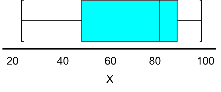
So, μ=71.7, and σ=28.4, and a box-whisker plot of the population data shown below indicates that the pain-function scores are somewhat skewed toward high scores.

Suppose we did not have the population data and instead we were estimating the mean functioning score in the population based on a sample of n=4. The table below shows all possible samples of size n=4 from the population of N=6, when sampling without replacement . The rightmost column shows the sample mean based on the 4 observations contained in that sample.
Table of Results of 15 Samples of 4 Each
|
Sample |
Observations in the Sample (n=4) |
Mean |
|||
|---|---|---|---|---|---|
|
1 |
25 |
50 |
80 |
85 |
60.0 |
|
2 |
25 |
50 |
80 |
90 |
61.3 |
|
3 |
25 |
50 |
80 |
100 |
63.6 |
|
4 |
25 |
50 |
85 |
90 |
62.5 |
|
5 |
25 |
50 |
85 |
100 |
65.0 |
|
6 |
25 |
59 |
90 |
100 |
66.3 |
|
7 |
25 |
80 |
85 |
90 |
70.0 |
|
8 |
25 |
80 |
85 |
100 |
72.5 |
|
9 |
25 |
80 |
90 |
100 |
73.8 |
|
10 |
25 |
85 |
90 |
100 |
75.0 |
|
11 |
50 |
80 |
85 |
90 |
76.3 |
|
12 |
50 |
80 |
85 |
100 |
78.8 |
|
13 |
50 |
80 |
90 |
100 |
80.0 |
|
14 |
50 |
85 |
90 |
100 |
81.3 |
|
15 |
80 |
85 |
90 |
100 |
88.8 |
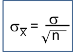
The collection of all possible sample means (in this example there are 15 distinct samples that are produced by sampling 4 individuals at random without replacement) is called the sampling distribution of the sample means, and we can consider it a population, because it includes all possible values produced by this sampling scheme. If we compute the mean and standard deviation of this population of sample means we get a mean = 71.7 and a standard deviation = 8.5. Notice also that the variability in the sample means is much smaller than the variability in the population, and the distribution of the sample means is more symmetric and has a much more restricted range than the distribution of the population data.


