The Role of Probability
Author:
Lisa Sullivan, PhD
Professor of Biostatistics
Boston University School of Public Health
Probabilities are numbers that reflect the likelihood that a particular event will occur. We hear about probabilities in many every-day situations ranging from weather forecasts (probability of rain or snow) to the lottery (probability of hitting the big jackpot). In biostatistical applications, it is probability theory that underlies statistical inference. Statistical inference involves making generalizations or inferences about unknown population parameters. After selecting a sample from the population of interest, we measure the characteristic under study, summarize this characteristic in our sample and then make inferences about the population based on what we observe in the sample. In this module we will discuss methods of sampling, basic concepts of probability, and applications of probability theory. In subsequent modules we will discuss statistical inference in detail and present methods that will enable you to make inferences about a population based on a single sample.
After completing this module, the student will be able to:

Note: Much of the content in the first half of this module is presented in a 38 minute lecture by Professor Lisa Sullivan. The lecture is available below, and a transcript of the lecture is also available. Link to transcript of lecture on basics probability
Sampling individuals from a population into a sample is a critically important step in any biostatistical analysis, because we are making generalizations about the population based on that sample. When selecting a sample from a population, it is important that the sample is representative of the population, i.e., the sample should be similar to the population with respect to key characteristics. For example, studies have shown that the prevalence of obesity is inversely related to educational attainment (i.e., persons with higher levels of education are less likely to be obese). Consequently, if we were to select a sample from a population in order to estimate the overall prevalence of obesity, we would want the educational level of the sample to be similar to that of the overall population in order to avoid an over- or underestimate of the prevalence of obesity.
There are two types of sampling: probability sampling and non-probability sampling. In probability sampling, each member of the population has a known probability of being selected. In non-probability sampling, each member of the population is selected without the use of probability.
In simple random sampling, one starts by identifying the sampling frame, i.e., a complete list or enumeration of all of the population elements (e.g., people, houses, phone numbers, etc.). Each of these is assigned a unique identification number, and elements are selected at random to determine the individuals to be included in the sample. As a result, each element has an equal chance of being selected, and the probability of being selected can be easily computed. This sampling strategy is most useful for small populations, because it requires a complete enumeration of the population as a first step.
Many introductory statistical textbooks contain tables of random numbers that can be used to ensure random selection, and statistical computing packages can be used to determine random numbers. Excel, for example, has a built-in function that can be used to generate random numbers.
Systematic sampling also begins with the complete sampling frame and assignment of unique identification numbers. However, in systematic sampling, subjects are selected at fixed intervals, e.g., every third or every fifth person is selected. The spacing or interval between selections is determined by the ratio of the population size to the sample size (N/n). For example, if the population size is N=1,000 and a sample size of n=100 is desired, then the sampling interval is 1,000/100 = 10, so every tenth person is selected into the sample. The selection process begins by selecting the first person at random from the first ten subjects in the sampling frame using a random number table; then 10th subject is selected.
If the desired sample size is n=175, then the sampling fraction is 1,000/175 = 5.7, so we round this down to five and take every fifth person. Once the first person is selected at random, every fifth person is selected from that point on through the end of the list.
With systematic sampling like this, it is possible to obtain non-representative samples if there is a systematic arrangement of individuals in the population. For example, suppose that the population of interest consisted of married couples and that the sampling frame was set up to list each husband and then his wife. Selecting every tenth person (or any even-numbered multiple) would result in selecting all males or females depending on the starting point. This is an extreme example, but one should consider all potential sources of systematic bias in the sampling process.
In stratified sampling, we split the population into non-overlapping groups or strata (e.g., men and women, people under 30 years of age and people 30 years of age and older), and then sample within each strata. The purpose is to ensure adequate representation of subjects in each stratum.
Sampling within each stratum can be by simple random sampling or systematic sampling. For example, if a population contains 70% men and 30% women, and we want to ensure the same representation in the sample, we can stratify and sample the numbers of men and women to ensure the same representation. For example, if the desired sample size is n=200, then n=140 men and n=60 women could be sampled either by simple random sampling or by systematic sampling.
There are many situations in which it is not possible to generate a sampling frame, and the probability that any individual is selected into the sample is unknown. What is most important, however, is selecting a sample that is representative of the population. In these situations non-probability samples can be used. Some examples of non-probability samples are described below.
In convenience sampling, we select individuals into our sample based on their availability to the investigators rather than selecting subjects at random from the entire population. As a result, the extent to which the sample is representative of the target population is not known. For example, we might approach patients seeking medical care at a particular hospital in a waiting or reception area. Convenience samples are useful for collecting preliminary or pilot data, but they should be used with caution for statistical inference, since they may not be representative of the target population.
In quota sampling, we determine a specific number of individuals to select into our sample in each of several specific groups. This is similar to stratified sampling in that we develop non-overlapping groups and sample a predetermined number of individuals within each. For example, suppose our desired sample size is n=300, and we wish to ensure that the distribution of subjects' ages in the sample is similar to that in the population. We know from census data that approximately 30% of the population are under age 20; 40% are between 20 and 49; and 30% are 50 years of age and older. We would then sample n=90 persons under age 20, n=120 between the ages of 20 and 49 and n=90 who are 50 years of age and older.
|
Age Group |
Distribution in Population |
Quota to Achieve n=300 |
|---|---|---|
|
<20 20-49 50+ |
30% 40% 30% |
n=90 n=120 n=90 |
Sampling proceeds until these totals, or quotas, are reached. Quota sampling is different from stratified sampling, because in a stratified sample individuals within each stratum are selected at random. Quota sampling achieves a representative age distribution, but it isn't a random sample, because the sampling frame is unknown. Therefore, the sample may not be representative of the population.
A probability is a number that reflects the chance or likelihood that a particular event will occur. Probabilities can be expressed as proportions that range from 0 to 1, and they can also be expressed as percentages ranging from 0% to 100%. A probability of 0 indicates that there is no chance that a particular event will occur, whereas a probability of 1 indicates that an event is certain to occur. A probability of 0.45 (45%) indicates that there are 45 chances out of 100 of the event occurring.
The concept of probability can be illustrated in the context of a study of obesity in children 5-10 years of age who are seeking medical care at a particular pediatric practice. The population (sampling frame) includes all children who were seen in the practice in the past 12 months and is summarized below.
|
|
Age (years) |
|
|||||
|
|
5 |
6 |
7 |
8 |
9 |
10 |
Total |
|
Boys |
432 |
379 |
501 |
410 |
420 |
418 |
2,560 |
|
Girls |
408 |
513 |
412 |
436 |
461 |
500 |
2,730 |
|
Totals |
840 |
892 |
913 |
846 |
881 |
918 |
5,290 |
If we select a child at random (by simple random sampling), then each child has the same probability (equal chance) of being selected, and the probability is 1/N, where N=the population size. Thus, the probability that any child is selected is 1/5,290 = 0.0002. In most sampling situations we are generally not concerned with sampling a specific individual but instead we concern ourselves with the probability of sampling certain types of individuals. For example, what is the probability of selecting a boy or a child 7 years of age? The following formula can be used to compute probabilities of selecting individuals with specific attributes or characteristics.
P(characteristic) = # persons with characteristic / N

Try to figure these out before looking at the answers:
Each of the probabilities computed in the previous section (e.g., P(boy), P(7 years of age)) is an unconditional probability, because the denominator for each is the total population size (N=5,290) reflecting the fact that everyone in the entire population is eligible to be selected. However, sometimes it is of interest to focus on a particular subset of the population (e.g., a sub-population). For example, suppose we are interested just in the girls and ask the question, what is the probability of selecting a 9 year old from the sub-population of girls? There is a total of NG=2,730 girls (here NG refers to the population of girls), and the probability of selecting a 9 year old from the sub-population of girls is written as follows:
P(9 year old | girls) = # persons with characteristic / N
where | girls indicates that we are conditioning the question to a specific subgroup, i.e., the subgroup specified to the right of the vertical line.
The conditional probability is computed using the same approach we used to compute unconditional probabilities. In this case:
P(9 year old | girls) = 461/2,730 = 0.169.
This also means that 16.9% of the girls are 9 years of age. Note that this is not the same as the probability of selecting a 9-year old girl from the overall population, which is P(girl who is 9 years of age) = 461/5,290 = 0.087.
What is the probability of selecting a boy from among the 6 year olds?
Answer
Screening tests are often used in clinical practice to assess the likelihood that a person has a particular medical condition. The rationale is that, if disease is identified early (before the manifestation of symptoms), then earlier treatment may lead to cure or improved survival or quality of life. This topic is also addressed in the core course in epidemiology in the learning module on Screening for Disease, in which one of the points that is stressed is that screening tests do not necessarily extend life or improve outcomes. In fact, many screening tests have potential adverse effects that need to be considered and weighed against the potential benefits. In addition, one needs to consider other factors when evaluating screening tests, such as their cost, availability, and discomfort.
Screening tests are often laboratory tests that detect particular markers of a specific disease. For example, the prostate-specific antigen (PSA) test for prostate cancer, which measures blood concentrations of PSA, a protein produced by the prostate gland. Many medical evaluations and tests may be thought of as screening procedures as well. For example, blood pressure tests, routine EKGs, breast exams, digital rectal exams, mammograms, routine blood and urine tests, or even questionnaires about behaviors and risk factors might all be considered screening tests. However, it is important to point out that none of these are definitive; they raise a heightened suspicion of disease, but they aren't diagnostic. A definitive diagnosis generally requires more extensive, sometimes invasive, and more reliable evaluations.
Nevertheless, let's return to the PSA test as an example of a screening test. In the absence of disease, levels of PSA are low, but elevated PSA levels can occur in the presence of prostate cancer, benign prostatic enlargement (a common condition in older men), and in the presence of infection or inflammation of the prostate gland. Thus, elevated levels of PSA may help identify men with prostate cancer, but they do not provide a definitive diagnosis, which requires biopsies of the prostate gland, in which tissue is sampled by a surgical procedure or by inserting a needle into the gland. The biopsy is then examined by a pathologist under a microscope, and based on the appearance of cells in the biopsy, a judgment is made as to whether the patient has prostate cancer or not. Obviously, if the screening test is to be useful clinically two conditions must be met. First, the test has to provide an advantage in distinguishing between, for example, men with and without prostate cancer. Second, one needs to demonstrate that early identification and treatment of the disease results in some improvement: a decreased probability of dying of the disease, or increased survival, or some measurable improvement in outcome.
One can collect data to examine the ability of a screening procedure to identify individuals with a disease. Suppose that a population of N=120 men over 50 years of age who are considered at high risk for prostate cancer have both the PSA screening test and a biopsy. The PSA results are reported as low, slightly to moderately elevated or highly elevated based on the following levels of measured protein, respectively: 0-2.5, 2.6-19.9 and 20 or more nanograms per milliliter.9 The biopsy results of the study are shown below.
|
PSA Level (Screening Test) |
Prostate Cancer |
No Prostate Cancer |
Totals |
|---|---|---|---|
|
Low (0-2.5 ng/ml) |
3 |
61 |
64 |
|
Slight/Moderate Elevation (2.6-19.9 ng/ml) |
13 |
28 |
41 |
|
Highly Elevated (>29 ng/ml) |
12 |
3 |
15 |
|
Totals |
28 |
92 |
120 |
Thus, the probability or likelihood that a man has prostate cancer is related to his PSA level. Based on these data, is the PSA test a clinically important screening test?
To address this question, let's first consider a screening test for Down Syndrome. In pregnancy, women often undergo screening to assess whether their fetus is likely to have Down Syndrome. The screening test evaluates levels of specific hormones in the blood. Screening test results are reported as positive or negative, indicating that a women is more or less likely to be carrying an affected fetus. Suppose that a population of N=4,810 pregnant women undergo the screening test and are scored as either positive or negative depending on the levels of hormones in the blood. In addition, suppose that each woman is followed to birth to determine whether the fetus was, in fact, affected with Down Syndrome. The results of the screening tests are summarized below.
|
Screening Test |
Down Syndrome |
No Down Syndrome |
Total |
|---|---|---|---|
|
Positive |
9 |
351 |
360 |
|
Negative |
1 |
4,449 |
4,450 |
|
Total |
10 |
4,800 |
4,810 |
In order to evaluate the screening test, each participant undergoes the screening test and is classified as positive or negative based on criteria that are specific to the test (e.g., high levels of a marker in a serum test or presence of a mass on a mammogram). A definitive diagnosis is also made for each participant based on definitive diagnostic tests or on an actual determination of outcome.
Using the data above, the probability that a woman with a positive screening test has an affected fetus is:
P(Affected Fetus | Screen Positive) = 9/360 = 0.025,
and the probability that a woman with a negative test has an affected fetus is
P(Affected Fetus | Negative Screen Positive) = 1/4,450 = 0.0002.
Is the serum screen a useful test?
As noted above, screening tests are not diagnostic, but instead may identify individuals more likely to have a certain condition. There are two measures that are commonly used to evaluate the performance of screening tests: the sensitivity and specificity of the test. The sensitivity of the test reflects the probability that the screening test will be positive among those who are diseased. In contrast, the specificity of the test reflects the probability that the screening test will be negative among those who, in fact, do not have the disease.
A total of N patients complete both the screening test and the diagnostic test. The data are often organized as follows with the results of the screening test shown in the rows and results of the diagnostic test are shown in the columns.
|
|
Diseased |
Disease Free |
Total |
|---|---|---|---|
|
Screen Positive |
a |
b |
a+b |
|
Screen Negative |
c |
d |
c+d |
|
|
a+c |
b+d |
N |
One might also consider the:
The false positive fraction is 1-specificity and the false negative fraction is 1-sensitivity. Therefore, knowing sensitivity and specificity captures the information in the false positive and false negative fractions. These are simply alternate ways of expressing the same information. Often times, sensitivity and the false positive fraction are reported for a test.
For the screening test for Down Syndrome the following results were obtained:
|
Screening Test Result |
Affected Fetus |
Unaffected Fetus |
Total |
|---|---|---|---|
|
Positive |
9 |
351 |
360 |
|
Negative |
1 |
4,449 |
4,450 |
|
Totals |
10 |
4,800 |
4,810 |
Thus, the performance characteristics of the test are:
However, the false positive and false negative fractions quantify errors in the test. The errors are often of greatest concern.
The sensitivity and false positive fractions are often reported for screening tests. However, for some tests, the specificity and false negative fractions might be the most important. The most important characteristics of any screening test depend on the implications of an error. In all cases, it is important to understand the performance characteristics of any screening test to appropriately interpret results and their implications.
Consider the results of a screening test from the patient's perspective! If the screening test is positive, the patient wants to know "What is the probability that I actually have the disease?" And if the test is negative, astute patients may ask, "What is the probability that I do not actually have disease if my test comes back negative?"
These questions refer to the positive and negative predictive values of the screening test, and they can be answered with conditional probabilities.
|
|
Diseased |
Non-Diseased |
Total |
|---|---|---|---|
|
Screen Positive |
a |
b |
a+b |
|
Screen Negative |
c |
d |
c+d |
|
Totals |
a+c |
b+d |
N |
Consider again the study evaluating pregnant women for carrying a fetus with Down Syndrome:
|
Screening Test |
Affected Fetus |
Unaffected Fetus |
Total |
|---|---|---|---|
|
Positive |
9 |
351 |
360 |
|
Negative |
1 |
4,449 |
4,450 |
|
Total |
10 |
4,800 |
4,810 |
The sensitivity and specificity of a screening test are characteristics of the test's performance at a given cut-off point (criterion of positivity). However, the positive predictive value of a screening test will be influenced not only by the sensitivity and specificity of the test, but also by the prevalence of the disease in the population that is being screened. In this example, the positive predictive value is very low (here 2.5%) because it depends on the prevalence of the disease in the population. This is due to the fact that as the disease becomes more prevalent, subjects are more frequently in the "affected" or "diseased" column, so the probability of disease among subjects with positive tests will be higher.
In this example, the prevalence of Down Syndrome in the population of N=4,810 women is 10/4,810 = 0.002 (i.e., in this population Down Syndrome affects 2 per 1,000 fetuses). While this screening test has good performance characteristics (sensitivity of 90.0% and specificity of 92.7%), the prevalence of the condition is low, so even a test with a high sensitivity and specificity has a low positive predictive value. Because positive and negative predictive values depend on the prevalence of the disease, they cannot be estimated in case control designs.
In probability, two events are said to be independent if the probability of one is not affected by the occurrence or non-occurrence of the other. This definition requires further explanation, so consider the following example.
Earlier in this module we considered data from a population of N=100 men who had both a PSA test and a biopsy for prostate cancer. Suppose we have a different test for prostate cancer. This prostate test produces a numerical risk that classifies a man as at low, moderate or high risk for prostate cancer. A sample of 100 men underwent the new test and also had a biopsy. The data from the biopsy results are summarized below.
| Prostate Test Risk |
Prostate Cancer |
No Prostate Cancer |
Total |
|---|---|---|---|
|
Low |
10 |
50 |
60 |
|
Moderate |
6 |
30 |
36 |
|
High |
4 |
20 |
24 |
|
|
20 |
100 |
120 |
Note that regardless of whether the hypothetical Prostate Test was low, moderate, or high, the probability that a subject had cancer was 0.167. In other words, knowing a man's prostate test result does not affect the likelihood that he has prostate cancer in this example. In this case, the probability that a man has prostate cancer is independent of his prostate test result.
Consider two events, call them A and B (e.g., A might be a low risk based on the "prostate test", and B is a diagnosis of prostate cancer). These two events are independent if P(A | B) = P(A) or if P(B | A) = P(B).
To check independence, we compare a conditional and an unconditional probability: P(A | B) = P(Low Risk | Prostate Cancer) = 10/20 = 0.50 and P(A) = P(Low Risk) = 60/120 = 0.50. The equality of the conditional and unconditional probabilities indicates independence.
Independence can also be tested by examining whether P(B | A) = P(Prostate Cancer | Low Risk) = 10/60 = 0.167 and P(B) = P(Prostate Cancer) = 20/120 = 0.167. In other words, the probability of the patient having a diagnosis of prostate cancer given a low risk "prostate test" (the conditional probability) is the same as the overall probability of having a diagnosis of prostate cancer (the unconditional probability).
Example:
The following table contains information on a population of N=6,732 individuals who are classified as having or not having prevalent cardiovascular disease (CVD). Each individual is also classified in terms of having a family history of cardiovascular disease. In this analysis, family history is defined as a first degree relative (parent or sibling) with diagnosed cardiovascular disease before age 60.
|
|
Prevalent CVD |
Free of CVD |
Total |
|---|---|---|---|
|
Family History of CVD |
491 |
368 |
859 |
|
No Family History of CVD |
152 |
5,721 |
5,873 |
|
Total |
643 |
6,089 |
6,732 |
Are family history and prevalent CVD independent? Is there a relationship between family history and prevalent CVD? This is a question of independence of events.
Let A=Prevalent CVD and B = Family History of CVD. (Note that it does not matter how we define A and B, for example we could have defined A=No Family History and B=Free of CVD, the result will be identical.) We now must check whether P(A | B) = P(A) or if P(B | A) = P(B). Again, it makes no difference which definition is used; the conclusion will be identical. We will compare the conditional probability to the unconditional probability as follows:
|
Conditional Probability |
Unconditional Probability |
|---|---|
|
P(A | B) = P(Prevalent CVD | Family History of CVD) = 491/859 = 0.572
The probability of prevalent CVD given a family history is 57.2% (as compared to 2.6% among patients with no family history). |
P(A) = P(Prevalent CVD) = 643/6,732 = 0.096
In the overall population, the probability of prevalent CVD is 9.6% (or 9.6% of the population has prevalent CVD). |
Since these probabilities are not equal, family history and prevalent CVD are not independent. Individuals with a family history of CVD are much more likely to have prevalent CVD.
Chris Wiggins, an associate professor of applied mathematics at Columbia University, posed the following question in an article in Scientific American: Link to the article in Scientific American:
"A patient goes to see a doctor. The doctor performs a test with 99 percent reliability--that is, 99 percent of people who are sick test positive and 99 percent of the healthy people test negative. The doctor knows that only 1 percent of the people in the country are sick. Now the question is: if the patient tests positive, what are the chances the patient is sick?"
The intuitive answer is 99 percent, but the correct answer is 50 percent...."
The solution to this question can easily be calculated using Bayes's theorem. Bayes, who was a reverend who lived from 1702 to 1761 stated that the probability you test positive AND are sick is the product of the likelihood that you test positive GIVEN that you are sick and the "prior" probability that you are sick (the prevalence in the population). Bayes's theorem allows one to compute a conditional probability based on the available information.
Bayes's Theorem
P(A) is the probability of event A
P(B) is the probability of event B
P(A|B) is the probability of observing event A if B is true
P(B|A) is the probability of observing event B if A is true.
Wiggins's explanation can be summarized with the help of the following table which illustrates the scenario in a hypothetical population of 10,000 people:
|
|
Diseased |
Not Diseased |
|
|---|---|---|---|
|
Test + |
99 |
99 |
198 |
|
Test - |
1 |
9,801 |
9,802 |
|
|
100 |
9,900 |
10,000 |
In this scenario P(A) is the unconditional probability of disease; here it is 100/10,000 = 0.01.
P(B) is the unconditional probability of a positive test; here it is 198/10,000 = 0.0198..
What we want to know is P (A | B), i.e., the probability of disease (A), given that the patient has a positive test (B). We know that prevalence of disease (the unconditional probability of disease) is 1% or 0.01; this is represented by P(A). Therefore, in a population of 10,000 there will be 100 diseased people and 9,900 non-diseased people. We also know the sensitivity of the test is 99%, i.e., P(B | A) = 0.99; therefore, among the 100 diseased people, 99 will test positive. We also know that the specificity is also 99%, or that there is a 1% error rate in non-diseased people. Therefore, among the 9,900 non-diseased people, 99 will have a positive test. And from these numbers, it follows that the unconditional probability of a positive test is 198/10,000 = 0.0198; this is P(B).
Thus, P(A | B) = (0.99 x 0.01) / 0.0198 = 0.50 = 50%.
From the table above, we can also see that given a positive test (subjects in the Test + row), the probability of disease is 99/198 = 0.05 = 50%.
Another Example:
Suppose a patient exhibits symptoms that make her physician concerned that she may have a particular disease. The disease is relatively rare in this population, with a prevalence of 0.2% (meaning it affects 2 out of every 1,000 persons). The physician recommends a screening test that costs $250 and requires a blood sample. Before agreeing to the screening test, the patient wants to know what will be learned from the test, specifically she wants to know the probability of disease, given a positive test result, i.e., P(Disease | Screen Positive).
The physician reports that the screening test is widely used and has a reported sensitivity of 85%. In addition, the test comes back positive 8% of the time and negative 92% of the time.
The information that is available is as follows:
Based on the available information, we could piece this together using a hypothetical population of 100,000 people. Given the available information this test would produce the results summarized in the table below. Point your mouse at the numbers in the table in order to get an explanation of how they were calculated.
|
|
Diseased |
Not Diseased |
|
|---|---|---|---|
|
Test + |
170 |
7,830 |
8,000 |
|
Test - |
30 |
91,970 |
92,000 |
|
|
200 |
99,800 |
100,000 |
The answer to the patient's question also could be computed from Bayes's Theorem:
We know that P(Disease)=0.002, P(Screen Positive | Disease)=0.85 and P(Screen Positive)=0.08. We can now substitute the values into the above equation to compute the desired probability,
P(Disease | Screen Positive) = (0.85)(0.002)/(0.08) = 0.021.
If the patient undergoes the test and it comes back positive, there is a 2.1% chance that he has the disease. Also, note, however, that without the test, there is a 0.2% chance that he has the disease (the prevalence in the population). In view of this, do you think the patient have the screening test?
Another important question that the patient might ask is, what is the chance of a false positive result? Specifically, what is P(Screen Positive| No Disease)? We can compute this conditional probability with the available information using Bayes Theorem.

By substituting the probabilities in this scenario, we get:

Thus, using Bayes Theorem, there is a 7.8% probability that the screening test will be positive in patients free of disease, which is the false positive fraction of the test.
Note that if P(Disease) = 0.002, then P(No Disease)=1-0.002. The events, Disease and No Disease, are called complementary events. The "No Disease" group includes all members of the population not in the "Disease" group. The sum of the probabilities of complementary events must equal 1 (i.e., P(Disease) + P(No Disease) = 1). Similarly, P(No Disease | Screen Positive) + P(Disease | Screen Positive) = 1.
To compute the probabilities in the previous section, we counted the number of participants that had a particular outcome or characteristic of interest, and divided by the population size. For conditional probabilities, the population size (denominator) was modified to reflect the sub-population of interest.
In each of the examples in the previous sections, we had a tabulation of the population (the sampling frame) that allowed us to compute the desired probabilities. However, there are instances in which a complete tabulation is not available. In some of these instances, probability models or mathematical equations can be used to generate probabilities. There are many probability models, and the model appropriate for a specific application depends on the specific attributes of the application. There are two particularly useful probability models:
These probability models are extremely important in statistical inference, and we will discuss these next.
The binomial distribution model is an important probability model that is used when there are two possible outcomes (hence "binomial"). In a situation in which there were more than two distinct outcomes, a multinomial probability model might be appropriate, but here we focus on the situation in which the outcome is dichotomous.
For example, adults with allergies might report relief with medication or not, children with a bacterial infection might respond to antibiotic therapy or not, adults who suffer a myocardial infarction might survive the heart attack or not, a medical device such as a coronary stent might be successfully implanted or not. These are just a few examples of applications or processes in which the outcome of interest has two possible values (i.e., it is dichotomous). The two outcomes are often labeled "success" and "failure" with success indicating the presence of the outcome of interest. Note, however, that for many medical and public health questions the outcome or event of interest is the occurrence of disease, which is obviously not really a success. Nevertheless, this terminology is typically used when discussing the binomial distribution model. As a result, whenever using the binomial distribution, we must clearly specify which outcome is the "success" and which is the "failure".
The binomial distribution model allows us to compute the probability of observing a specified number of "successes" when the process is repeated a specific number of times (e.g., in a set of patients) and the outcome for a given patient is either a success or a failure. We must first introduce some notation which is necessary for the binomial distribution model.
First, we let "n" denote the number of observations or the number of times the process is repeated, and "x" denotes the number of "successes" or events of interest occurring during "n" observations. The probability of "success" or occurrence of the outcome of interest is indicated by "p".
The binomial equation also uses factorials. In mathematics, the factorial of a non-negative integer k is denoted by k!, which is the product of all positive integers less than or equal to k. For example,
With this notation in mind, the binomial distribution model is defined as:
The Binomial Distribution Model
Use of the binomial distribution requires three assumptions:
For a more intuitive explanation of the binomial distribution, you might want to watch the following video from KhanAcademy.org.
Suppose that 80% of adults with allergies report symptomatic relief with a specific medication. If the medication is given to 10 new patients with allergies, what is the probability that it is effective in exactly seven?
First, do we satisfy the three assumptions of the binomial distribution model?
We know that:
The probability of 7 successes is:
This is equivalent to:

But many of the terms in the numerator and denominator cancel each other out,
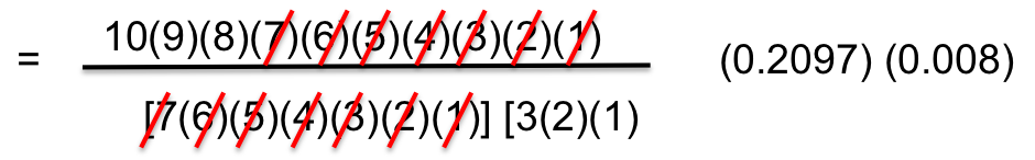
so this can be simplified to:

Interpretation: There is a 20.13% probability that exactly 7 of 10 patients will report relief from symptoms when the probability that any one reports relief is 80%.

Note: Binomial probabilities like this can also be computed in an Excel spreadsheet using the =BINOMDIST function. Place the cursor into an empty cell and enter the following formula:
=BINOMDIST(x,n,p,FALSE)
where x= # of 'successes', n = # of replications or observations, and p = probability of success on a single observation.
What is the probability that none report relief? We can again use the binomial distribution model with n=10, x=0 and p=0.80.
This is equivalent to
whixh simpliefies to

Interpretation: There is practically no chance that none of the 10 will report relief from symptoms when the probability of reporting relief for any individual patient is 80%.
What is the most likely number of patients who will report relief out of 10? If 80% report relief and we consider 10 patients, we would expect that 8 report relief. What is the probability that exactly 8 of 10 report relief? We can use the same method that was used above to demonstrate that there is a 30.30% probability that exactly 8 of 10 patients will report relief from symptoms when the probability that any one reports relief is 80%. The probability that exactly 8 report relief will be the highest probability of all possible outcomes (0 through 10).
The likelihood that a patient with a heart attack dies of the attack is 0.04 (i.e., 4 of 100 die of the attack). Suppose we have 5 patients who suffer a heart attack, what is the probability that all will survive? For this example, we will call a success a fatal attack (p = 0.04). We have n=5 patients and want to know the probability that all survive or, in other words, that none are fatal (0 successes).
We again need to assess the assumptions. Each attack is fatal or non-fatal, the probability of a fatal attack is 4% for all patients and the outcome of individual patients are independent. It should be noted that the assumption that the probability of success applies to all patients must be evaluated carefully. The probability that a patient dies from a heart attack depends on many factors including age, the severity of the attack, and other comorbid conditions. To apply the 4% probability we must be convinced that all patients are at the same risk of a fatal attack. The assumption of independence of events must also be evaluated carefully. As long as the patients are unrelated, the assumption is usually appropriate. Prognosis of disease could be related or correlated in members of the same family or in individuals who are co-habitating. In this example, suppose that the 5 patients being analyzed are unrelated, of similar age and free of comorbid conditions.

There is an 81.54% probability that all patients will survive the attack when the probability that any one dies is 4%. In this example, the possible outcomes are 0, 1, 2, 3, 4 or 5 successes (fatalities). Because the probability of fatality is so low, the most likely response is 0 (all patients survive). The binomial formula generates the probability of observing exactly x successes out of n.
If we want to compute the probability of a range of outcomes we need to apply the formula more than once. Suppose in the heart attack example we wanted to compute the probability that no more than 1 person dies of the heart attack. In other words, 0 or 1, but not more than 1. Specifically we want P(no more than 1 success) = P(0 or 1 successes) = P(0 successes) + P(1 success). To solve this probability we apply the binomial formula twice.
We already computed P(0 successes), we now compute P(1 success):

P(no more than 1 'success') = P(0 or 1 successes) = P(0 successes) + P(1 success)
= 0.8154 + 0.1697 = 0.9851.
The probability that no more than 1 of 5 (or equivalently that at most 1 of 5) die from the attack is 98.51%.
What is the probability that 2 or more of 5 die from the attack? Here we want to compute P(2 or more successes). The possible outcomes are 0, 1, 2, 3, 4 or 5, and the sum of the probabilities of each of these outcomes is 1 (i.e., we are certain to observe either 0, 1, 2, 3, 4 or 5 successes). We just computed P(0 or 1 successes) = 0.9851, so P(2, 3, 4 or 5 successes) = 1 - P(0 or 1 successes) = 0.0149. There is a 1.49% probability that 2 or more of 5 will die from the attack.
Mean number of successes: 
Standard Deviation: 
For the previouos example on the probability of relief from allergies with n-10 trialsand p=0.80 probability of success on each trial:

Suppose you flipped a coin 10 times (i.e., 10 trials), and the probability of getting "heads" was 0.5 (50%). What would be the probability of getting exactly 4 heasds?
ANSWER
|
With 4 successes, 10 trials, and probability =0.5 on each trial What is the : |
Probability |
R coding to compute these |
|---|---|---|
| a) Probability of exactly 4 events = | 0.205078 |
> dbinom (4, 10, 0.5) |
| b) Cumulative probability of < 4 events = | 0.171875 |
> pbinom (3, 10, 0.5, lower.tail=TRUE) |
| c) Cumulative probability of < 4 events = | 0.376953 |
> pbinom(4, 10, 0.5, lower.tail=TRUE) |
| d) Cumulative probability of > 4 events = | 0.623047 |
> pbinom(4, 10, 0.5, lower.tail=FALSE) |
| e) Cumulative probability of > 4 events = | 0.828125 |
pbinom (3, 10, 0.5, lower.tail=FALSE) |
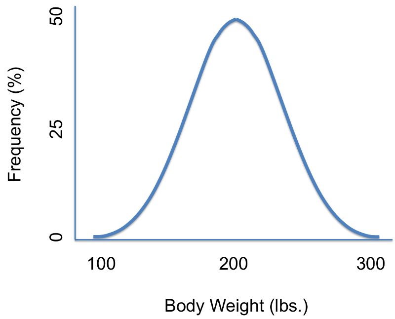
Suppose we were interested in characterizing the variability in body weights among adults in a population. We could measure each subject's weight and then summarize our findings with a graph that displays different body weights on the horizontal axis (the X-axis) and the frequency (% of subjects) of each weight on the vertical axis (the Y-axis) as shown in the illustration on the left. There are several noteworthy characteristics of this graph. It is bell-shaped with a single peak in the center, and it is symmetrical. If the distribution is perfectly symmetrical with a single peak in the center, then the mean value, the mode, and the median will be all be the same. Many variables have similar characteristics, which are characteristic of so-called normal or Gaussian distributions. Note that the horizontal or X-axis displays the scale of the characteristic being analyzed (in this case weight), while the height of the curve reflects the probability of observing each value. The fact that the curve is highest in the middle suggests that the middle values have higher probability or are more likely to occur, and the curve tails off above and below the middle suggesting that values at either extreme are much less likely to occur. There are different probability models for continuous outcomes, and the appropriate model depends on the distribution of the outcome of interest. The normal probability model applies when the distribution of the continuous outcome conforms reasonably well to a normal or Gaussian distribution, which resembles a bell shaped curve. Note normal probability model can be used even if the distribution of the continuous outcome is not perfectly symmetrical; it just has to be reasonably close to a normal or Gaussian distribution.
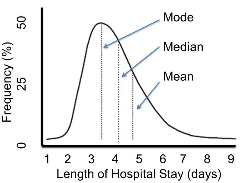
However, other distributions do not follow the symmetrical patterns shown above. For example, if we were to study hospital admissions and the number of days that admitted patients spend in the hospital, we would find that the distribution was not symmetrical, but skewed. Note that the distribution to the distribution below is not symmetrical, and the mean value is not the same as the mode or the median.
Distributions that are normal or Gaussian have the following characteristics:
If we have a normally distributed variable and know the population mean (μ) and the standard deviation (σ), then we can compute the probability of particular values based on this equation for the normal probability model:
where μ is the population mean and σ is the population standard deviation. (π is a constant = 3.14159, and e is a constant = 2.71828.) Normal probabilities can be calculated using calculus or from an Excel spreadsheet (see the normal probability calculator further down the page. There are also very useful tables that list the probabilities.
Consider body mass index (BMI) in a population of 60 year old males in whom BMI is normally distributed and has a mean value = 29 and a standard deviation = 6. The standard deviation gives us a measure of how spread out the observations are.
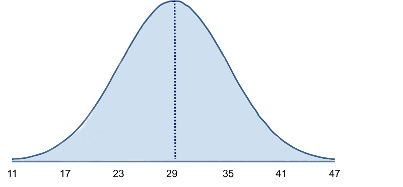
The mean (μ = 29) is in the center of the distribution, and the horizontal axis is scaled in increments of the standard deviation (σ = 6) and the distribution essentially ranges from μ - 3 σ to μ + 3σ. It is possible to have BMI values below 11 or above 47, but extreme values occur very infrequently. To compute probabilities from normal distributions, we will compute areas under the curve. For any probability distribution, the total area under the curve is 1. For the normal distribution, we know that the mean is equal to median, so half (50%) of the area under the curve is above the mean and half is below, so P(BMI < 29)=0.50. Consequently, if we select a man at random from this population and ask what is the probability his BMI is less than 29?, the answer is 0.50 or 50%, since 50% of the area under the curve is below the value BMI = 29. Note that with the normal distribution the probability of having any exact value is 0 because there is no area at an exact BMI value, so in this case, the probability that his BMI = 29 is 0, but the probability that his BMI is <29 or the probability that his BMI is < 29 is 50%.
What is the probability that a 60 year old male has BMI less than 35? The probability is displayed graphically and represented by the area under the curve to the left of the value 35 in the figure below.
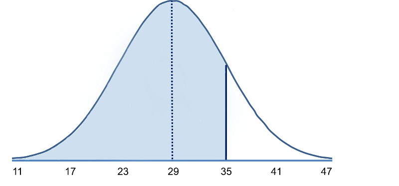
Note that BMI = 35 is 1 standard deviation above the mean. For the normal distribution we know that approximately 68% of the area under the curve lies between the mean plus or minus one standard deviation. Therefore, 68% of the area under the curve lies between 23 and 35. We also know that the normal distribution is symmetric about the mean, therefore P(29 < X < 35) = P(23 < X < 29) = 0.34. Consequently, P(X < 35) = 0.5 + 0.34 = 0.84. [In other words, 68% of the area is between 23 and 35, so 34% of the area is between 29-35, and 50% is below 29. If the total area under the curve is 1, then the area below 35 = ).50 + 0.34 = 0.84 or 84%.
What is the probability that a 60 year old male has BMI less than 41? [Hint: A BMI of 41 is 2 standard deviations above the mean.] Try to figure this out on your own before looking at the answer.
Answer
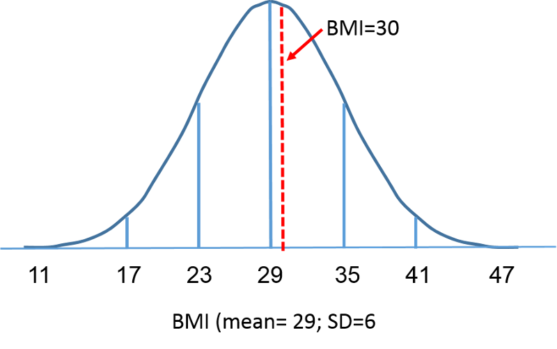
It is easy to figure out the probabilities for values that are increments of the standard deviation above or below the mean, but what if the value isn't an exact multiple of the standard deviation? For example, suppose we want to compute the probability that a randomly selected male has a BMI less than 30 (which is the threshold for classifying someone as obese).
Because 30 is neither the mean nor a multiple of standard deviations above or below the mean, we cannot simply use the probabilities known to be associated with 1, 2, or 3 standard deviations from the mean. In a sense, we need to know how far a given value is from the mean and the probability of having values less than this. And, of course, we would want to have a way of figuring this out not only for BMI values in a population of males with a mean of 29 and a standard deviation of 6, but for any normally distributed variable. So, what we need is a standardized way of evaluating any normally distributed data so that we can compute the probability of observing the results obtained from samples that we take. We can do all of this fairly easily by using a "standard normal distribution."
We were looking at body mass index (BMI) in a population of 60 year old males in whom BMI was normally distributed and had a mean value = 29 and a standard deviation = 6.
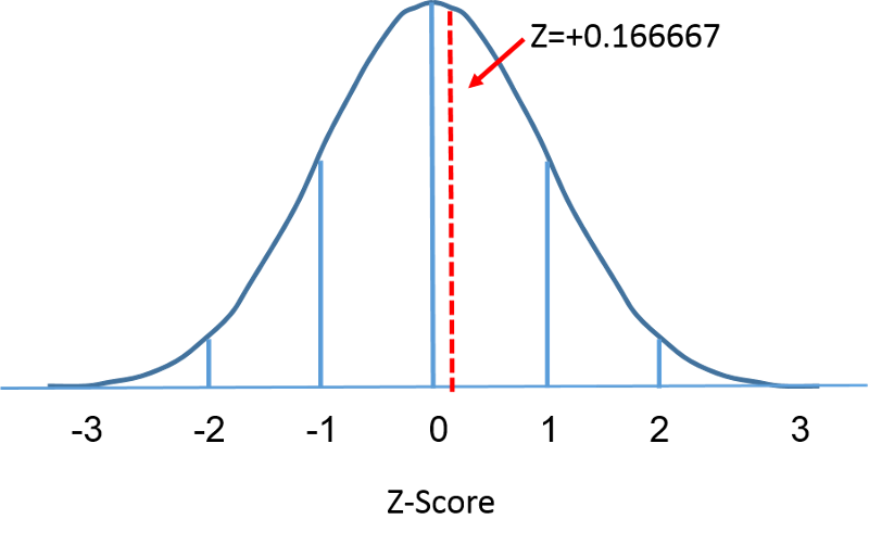
What is the probability that a randomly selected male from this population would have a BMI less than 30?" While a value of 30 doesn't fall on one of the increments of standard deviation, we can caculate how many standard deviaton it is away from the mean.
It is 30-29=1 BMI unit above the means. The standard deviation is 6, so 1 BMI unit above the mean is1/6 = 0.166667 standard deviations above the mean.This provides us with a way of standardizing how far a given observation is from the mean for any normal distribution, regardless of its mean or standard deviation. Now what we need is a way of finding the probabilities associated various Z-scores. This can be done by using the standard normal distribution as described on the next page.
The standard normal distribution is a normal distribution with a mean of zero and standard deviation of 1. The standard normal distribution is centered at zero and the degree to which a given measurement deviates from the mean is given by the standard deviation. For the standard normal distribution, 68% of the observations lie within 1 standard deviation of the mean; 95% lie within two standard deviation of the mean; and 99.9% lie within 3 standard deviations of the mean. To this point, we have been using "X" to denote the variable of interest (e.g., X=BMI, X=height, X=weight). However, when using a standard normal distribution, we will use "Z" to refer to a variable in the context of a standard normal distribution. After standarization, the BMI=30 discussed on the previous page is shown below lying 0.16667 units above the mean of 0 on the standard normal distribution on the right.
 ====
====
Since the area under the standard curve = 1, we can begin to more precisely define the probabilities of specific observation. For any given Z-score we can compute the area under the curve to the left of that Z-score. The table in the frame below shows the probabilities for the standard normal distribution. Examine the table and note that a "Z" score of 0.0 lists a probability of 0.50 or 50%, and a "Z" score of 1, meaning one standard deviation above the mean, lists a probability of 0.8413 or 84%. That is because one standard deviation above and below the mean encompasses about 68% of the area, so one standard deviation above the mean represents half of that of 34%. So, the 50% below the mean plus the 34% above the mean gives us 84%.
This table is organized to provide the area under the curve to the left of or less of a specified value or "Z value". In this case, because the mean is zero and the standard deviation is 1, the Z value is the number of standard deviation units away from the mean, and the area is the probability of observing a value less than that particular Z value. Note also that the table shows probabilities to two decimal places of Z. The units place and the first decimal place are shown in the left hand column, and the second decimal place is displayed across the top row.
But let's get back to the question about the probability that the BMI is less than 30, i.e., P(X<30). We can answer this question using the standard normal distribution. The figures below show the distributions of BMI for men aged 60 and the standard normal distribution side-by-side.
Distribution of BMI and Standard Normal Distribution
====
The area under each curve is one but the scaling of the X axis is different. Note, however, that the areas to the left of the dashed line are the same. The BMI distribution ranges from 11 to 47, while the standardized normal distribution, Z, ranges from -3 to 3. We want to compute P(X < 30). To do this we can determine the Z value that corresponds to X = 30 and then use the standard normal distribution table above to find the probability or area under the curve. The following formula converts an X value into a Z score, also called a standardized score:

where μ is the mean and σ is the standard deviation of the variable X.
In order to compute P(X < 30) we convert the X=30 to its corresponding Z score (this is called standardizing):
Thus, P(X < 30) = P(Z < 0.17). We can then look up the corresponding probability for this Z score from the standard normal distribution table, which shows that P(X < 30) = P(Z < 0.17) = 0.5675. Thus, the probability that a male aged 60 has BMI less than 30 is 56.75%.
Another Example
Using the same distribution for BMI, what is the probability that a male aged 60 has BMI exceeding 35? In other words, what is P(X > 35)? Again we standardize:
We now go to the standard normal distribution table to look up P(Z>1) and for Z=1.00 we find that P(Z<1.00) = 0.8413. Note, however, that the table always gives the probability that Z is less than the specified value, i.e., it gives us P(Z<1)=0.8413.
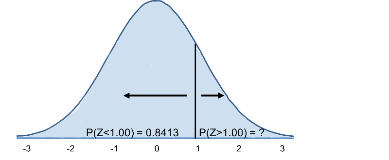
Therefore, P(Z>1)=1-0.8413=0.1587. Interpretation: Almost 16% of men aged 60 have BMI over 35.
As an alternative to looking up normal probabilities in the table or using Excel, we can use R to compute probabilities. For example,
> pnorm(0)
[1] 0.5
A Z-score of 0 (the mean of any distribution) has 50% of the area to the left. What is the probability that a 60 year old man in the population above has a BMI less than 29 (the mean)? The Z-score would be 0, and pnorm(0)=0.5 or 50%.
What is the probability that a 60 year old man will have a BMI less than 30? The Z-score was 0.16667.
> pnorm(0.16667)
[1] 0.5661851
So, the probabilty is 56.6%.
What is the probability that a 60 year old man will have a BMI greater than 35?
35-29=6, which is one standard deviation above the mean. So we can compute the area to the left
> pnorm(1)
[1] 0.8413447
and then subtract the result from 1.0.
1-0.8413447= 0.1586553
So the probability of a 60 year ld man having a BMI greater than 35 is 15.8%.
Or, we can use R to compute the entire thing in a single step as follows:
> 1-pnorm(1)
[1] 0.1586553
What is the probability that a male aged 60 has BMI between 30 and 35? Note that this is the same as asking what proportion of men aged 60 have BMI between 30 and 35. Specifically, we want P(30 < X < 35)? We previously computed P(30<X) and P(X<35); how can these two results be used to compute the probability that BMI will be between 30 and 35? Try to formulate and answer on your own before looking at the explanation below.
Answer
Now consider BMI in women. What is the probability that a female aged 60 has BMI less than 30? We use the same approach, but for women aged 60 the mean is 28 and the standard deviation is 7.
Answer
What is the probability that a female aged 60 has BMI exceeding 40? Specifically, what is P(X > 40)?
Answer
The standard normal distribution can also be useful for computing percentiles. For example, the median is the 50th percentile, the first quartile is the 25th percentile, and the third quartile is the 75th percentile. In some instances it may be of interest to compute other percentiles, for example the 5th or 95th. The formula below is used to compute percentiles of a normal distribution.

where μ is the mean and σ is the standard deviation of the variable X, and Z is the value from the standard normal distribution for the desired percentile.
Example:
What is the 90th percentile of BMI for men?
The 90th percentile is the BMI that holds 90% of the BMIs below it and 10% above it, as illustrated in the figure below.
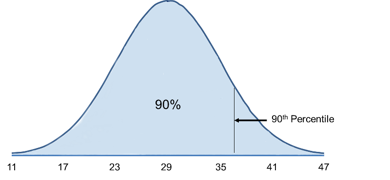
To compute the 90th percentile, we use the formula X=μ + Zσ, and we will use the standard normal distribution table, except that we will work in the opposite direction. Previously we started with a particular "X" and used the table to find the probability. However, in this case we want to start with a 90% probability and find the value of "X" that represents it.
So we begin by going into the interior of the standard normal distribution table to find the area under the curve closest to 0.90, and from this we can determine the corresponding Z score. Once we have this we can use the equation X=μ + Zσ, because we already know that the mean and standard deviation are 29 and 6, respectively.
When we go to the table, we find that the value 0.90 is not there exactly, however, the values 0.8997 and 0.9015 are there and correspond to Z values of 1.28 and 1.29, respectively (i.e., 89.97% of the area under the standard normal curve is below 1.28). The exact Z value holding 90% of the values below it is 1.282 which was determined from a table of standard normal probabilities with more precision.
Using Z=1.282 the 90th percentile of BMI for men is: X = 29 + 1.282(6) = 36.69.
Interpretation: Ninety percent of the BMIs in men aged 60 are below 36.69. Ten percent of the BMIs in men aged 60 are above 36.69.
What is the 90th percentile of BMI among women aged 60? Recall that the mean BMI for women aged 60 the mean is 28 with a standard deviation of 7.
Answer
The table below shows Z values for commonly used percentiles.
|
Percentile |
Z |
|---|---|
|
1st |
-2.326 |
|
2.5th |
-1.960 |
|
5th |
-1.645 |
|
10th |
-1.282 |
|
25th |
-0.675 |
|
50th |
0 |
|
75th |
0.675 |
|
90th |
1.282 |
|
95th |
1.645 |
|
97.5th |
1.960 |
|
99th |
2.326 |
Percentiles of height and weight are used by pediatricians in order to evaluate development relative to children of the same sex and age. For example, if a child's weight for age is extremely low it might be an indication of malnutrition. Growth charts are available at http://www.cdc.gov/growthcharts/.
For infant girls, the mean body length at 10 months is 72 centimeters with a standard deviation of 3 centimeters. Suppose a girl of 10 months has a measured length of 67 centimeters. How does her length compare to other girls of 10 months?
Answer
A complete blood count (CBC) is a commonly performed test. One component of the CBC is the white blood cell (WBC) count, which may be indicative of infection if the count is high. WBC counts are approximately normally distributed in healthy people with a mean of 7550 WBC per mm3 (i.e., per microliter) and a standard deviation of 1085. What proportion of subjects have WBC counts exceeding 9000?
Answer
Using the mean and standard deviation in the previous question, what proportion of patients have WBC counts between 5000 and 7000?
Answer
If the top 10% of WBC counts are considered abnormal, what is the upper limit of normal?
Answer
The mean of a representative sample provides an estimate of the unknown population mean, but intuitively we know that if we took multiple samples from the same population, the estimates would vary from one another. We could, in fact, sample over and over from the same population and compute a mean for each of the samples. In essence, all these sample means constitute yet another "population," and we could graphically display the frequency distribution of the sample means. This is referred to as the sampling distribution of the sample means.
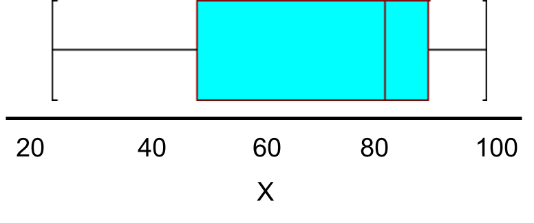
Consider the following small population consisting of N=6 patients who recently underwent total hip replacement. Three months after surgery they rated their pain-free function on a scale of 0 to 100 (0=severely limited and painful functioning to 100=completely pain free functioning). The data are shown below and ordered from smallest to largest.
Pain-Free Function Ratings in a Small Population of N=6 Patients:
25, 50, 80, 85, 90, 100
The population mean is
The population standard deviation is
So, μ=71.7, and σ=28.4, and a box-whisker plot of the population data shown below indicates that the pain-function scores are somewhat skewed toward high scores.
Suppose we did not have the population data and instead we were estimating the mean functioning score in the population based on a sample of n=4. The table below shows all possible samples of size n=4 from the population of N=6, when sampling without replacement. The rightmost column shows the sample mean based on the 4 observations contained in that sample.
Table of Results of 15 Samples of 4 Each
|
Sample |
Observations in the Sample (n=4) |
Mean |
|||
|---|---|---|---|---|---|
|
1 |
25 |
50 |
80 |
85 |
60.0 |
|
2 |
25 |
50 |
80 |
90 |
61.3 |
|
3 |
25 |
50 |
80 |
100 |
63.6 |
|
4 |
25 |
50 |
85 |
90 |
62.5 |
|
5 |
25 |
50 |
85 |
100 |
65.0 |
|
6 |
25 |
59 |
90 |
100 |
66.3 |
|
7 |
25 |
80 |
85 |
90 |
70.0 |
|
8 |
25 |
80 |
85 |
100 |
72.5 |
|
9 |
25 |
80 |
90 |
100 |
73.8 |
|
10 |
25 |
85 |
90 |
100 |
75.0 |
|
11 |
50 |
80 |
85 |
90 |
76.3 |
|
12 |
50 |
80 |
85 |
100 |
78.8 |
|
13 |
50 |
80 |
90 |
100 |
80.0 |
|
14 |
50 |
85 |
90 |
100 |
81.3 |
|
15 |
80 |
85 |
90 |
100 |
88.8 |
The collection of all possible sample means (in this example there are 15 distinct samples that are produced by sampling 4 individuals at random without replacement) is called the sampling distribution of the sample means, and we can consider it a population, because it includes all possible values produced by this sampling scheme. If we compute the mean and standard deviation of this population of sample means we get a mean = 71.7 and a standard deviation = 8.5. Notice also that the variability in the sample means is much smaller than the variability in the population, and the distribution of the sample means is more symmetric and has a much more restricted range than the distribution of the population data.

The central limit theorem states that if you have a population with mean μ and standard deviation σ and take sufficiently large random samples from the population with replacement, then the distribution of the sample means will be approximately normally distributed. This will hold true regardless of whether the source population is normal or skewed, provided the sample size is sufficiently large (usually n > 30). If the population is normal, then the theorem holds true even for samples smaller than 30. In fact, this also holds true even if the population is binomial, provided that min(np, n(1-p))> 5, where n is the sample size and p is the probability of success in the population. This means that we can use the normal probability model to quantify uncertainty when making inferences about a population mean based on the sample mean.
For the random samples we take from the population, we can compute the mean of the sample means:

and the standard deviation of the sample means:

Before illustrating the use of the Central Limit Theorem (CLT) we will first illustrate the result. In order for the result of the CLT to hold, the sample must be sufficiently large (n > 30). Again, there are two exceptions to this. If the population is normal, then the result holds for samples of any size (i..e, the sampling distribution of the sample means will be approximately normal even for samples of size less than 30).
The figure below illustrates a normally distributed characteristic, X, in a population in which the population mean is 75 with a standard deviation of 8.
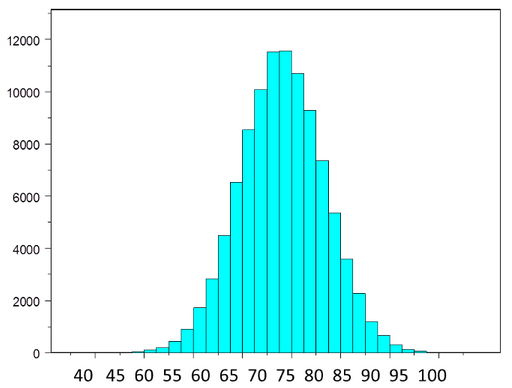
If we take simple random samples (with replacement) of size n=10 from the population and compute the mean for each of the samples, the distribution of sample means should be approximately normal according to the Central Limit Theorem. Note that the sample size (n=10) is less than 30, but the source population is normally distributed, so this is not a problem. The distribution of the sample means is illustrated below. Note that the horizontal axis is different from the previous illustration, and that the range is narrower.
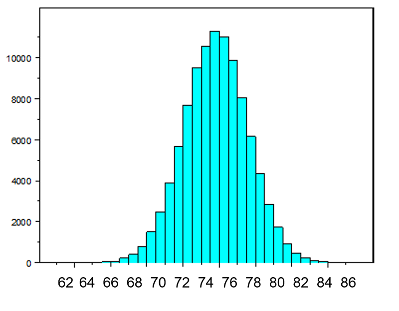
The mean of the sample means is 75 and the standard deviation of the sample means is 2.5, with the standard deviation of the sample means computed as follows:
If we were to take samples of n=5 instead of n=10, we would get a similar distribution, but the variation among the sample means would be larger. In fact, when we did this we got a sample mean = 75 and a sample standard deviation = 3.6.
Now suppose we measure a characteristic, X, in a population and that this characteristic is dichotomous (e.g., success of a medical procedure: yes or no) with 30% of the population classified as a success (i.e., p=0.30) as shown below.
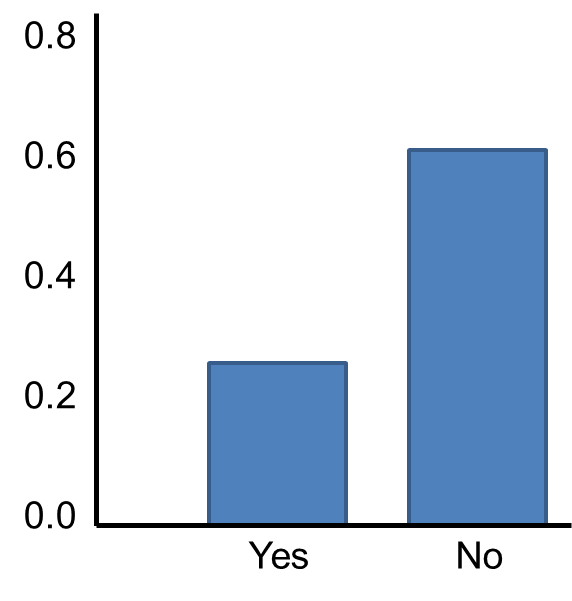
The Central Limit Theorem applies even to binomial populations like this provided that the minimum of np and n(1-p) is at least 5, where "n" refers to the sample size, and "p" is the probability of "success" on any given trial. In this case, we will take samples of n=20 with replacement, so min(np, n(1-p)) = min(20(0.3), 20(0.7)) = min(6, 14) = 6. Therefore, the criterion is met.
We saw previously that the population mean and standard deviation for a binomial distribution are:
Mean binomial probability:
Standard deviation: 
The distribution of sample means based on samples of size n=20 is shown below.
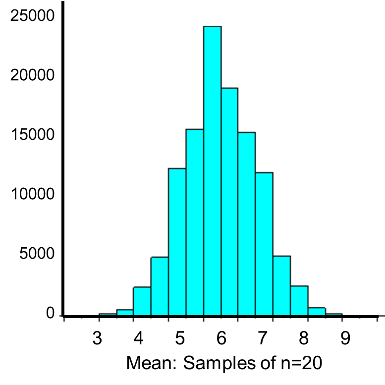
The mean of the sample means is
and the standard deviation of the sample means is:
Now, instead of taking samples of n=20, suppose we take simple random samples (with replacement) of size n=10. Note that in this scenario we do not meet the sample size requirement for the Central Limit Theorem (i.e., min(np, n(1-p)) = min(10(0.3), 10(0.7)) = min(3, 7) = 3).The distribution of sample means based on samples of size n=10 is shown on the right, and you can see that it is not quite normally distributed. The sample size must be larger in order for the distribution to approach normality.
The Poisson distribution is another probability model that is useful for modeling discrete variables such as the number of events occurring during a given time interval. For example, suppose you typically receive about 4 spam emails per day, but the number varies from day to day. Today you happened to receive 5 spam emails. What is the probability of that happening, given that the typical rate is 4 per day? The Poisson probability is:
Mean = μ
Standard deviation = 
The mean for the distribution is μ (the average or typical rate), "X" is the actual number of events that occur ("successes"), and "e" is the constant approximately equal to 2.71828. So, in the example above
Now let's consider another Poisson distribution. with μ=3 and σ=1.73. The distribution is shown in the figure below.
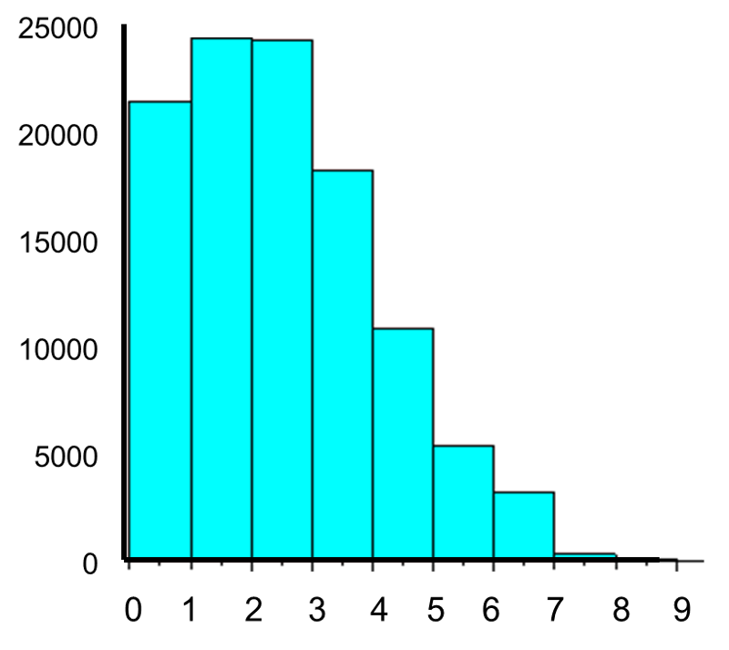
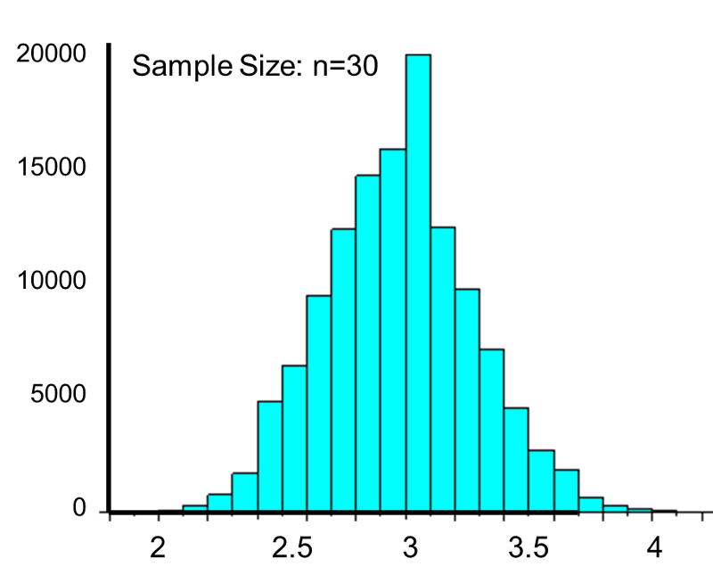
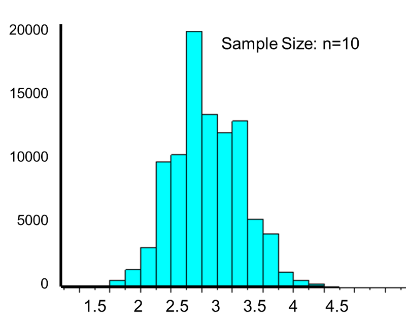
This population is not normally distributed, but the Central Limit Theorem will apply if n > 30. In fact, if we take samples of size n=30, we obtain samples distributed as shown in the first graph below with a mean of 3 and standard deviation = 0.32. In contrast, with small samples of n=10, we obtain samples distributed as shown in the lower graph. Note that n=10 does not meet the criterion for the Central Limit Theorem, and the small samples on the right give a distribution that is not quite normal. Also note that the sample standard deviation (also called the "standard error") is larger with smaller samples, because it is obtained by dividing the population standard deviation by the square root of the sample size. Another way of thinking about this is that extreme values will have less impact on the sample mean when the sample size is large.
Cholesterol molecules are transported in blood by large macromolecular assemblies (illustrated below) called lipoproteins that are really a conglomerate of molecules including apolipoproteins, phospholipids, cholesterol, and cholesterol esters. This macromolecular carrier particles make it possible to transport lipid molecules in blood, which is essentially an aqueous system.
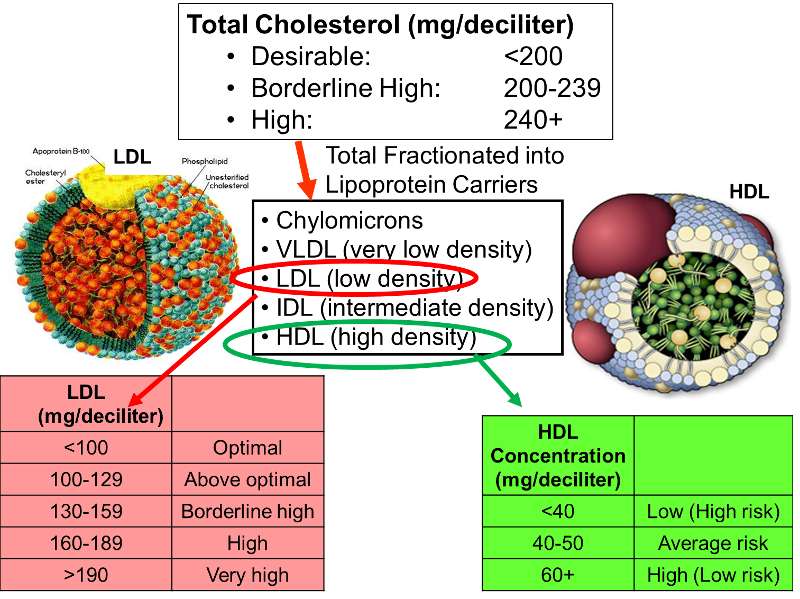
Different classes of these lipid transport carriers can be separated (fractionated)based on their density and where they layer out when spun in a centrifuge. High density lipoprotein cholesterol (HDL) is sometimes referred to as the "good cholesterol," because higher concentrations of HDL in blood are associated with a lower risk of coronary heart disease. In contrast, high concentrations of low density lipoprotein cholesterol (LDL) are associated with an increased risk of coronary heart disease. The illustration on the right outlines how total cholesterol levels are classified in terms of risk, and how the levels of LDL and HDL fractions provide additional information regarding risk.
Example:
Data from the Framingham Heart Study found that subjects over age 50 had a mean HDL of 54 and a standard deviation of 17. Suppose a physician has 40 patients over age 50 and wants to determine the probability that the mean HDL cholesterol for this sample of 40 men is 60 mg/dl or more (i.e., low risk). Probability questions about a sample mean can be addressed with the Central Limit Theorem, as long as the sample size is sufficiently large. In this case n=40, so the sample mean is likely to be approximately normally distributed, so we can compute the probability of HDL>60 by using the standard normal distribution table.
The population mean is 54, but the question is what is the probability that the sample mean will be >60?
In general,

the standard deviation of the sample mean is

Therefore, the formula to standardize a sample mean is:
And in this case:
P(Z > 2.22) can be looked up in the standard normal distribution table, and because we want the probability that P(Z > 2.22), we compute is as P(Z > 2.22) = 1 - 0.9868 = 0.0132.
Therefore, the probability that the mean HDL in these 40 patients will exceed 60 is 1.32%.
What is the probability that the mean HDL cholesterol among these 40 patients is less than 50?
Answer
Example:
Suppose we want to estimate the mean LDL cholesterol) in the population of adults 65 years of age and older. We know from studies of adults under age 65 that the standard deviation is 13, and we will assume that the variability in LDL in adults 65 years of age and older is the same. We will select a sample of n=100 participants > 65 years of age, and we will use the mean of the sample as an estimate of the population mean. We want our estimate to be precise, specifically we want it to be within 3 units of the true mean LDL value. What is the probability that our estimate (i.e., the sample mean) will be within 3 units of the true mean? We think of this question as P(μ - 3 < sample mean < μ + 3).
Because this is a probability about a sample mean, we will use the Central Limit Theorem. With a sample of size n=100 we clearly satisfy the sample size criterion so we can use the Central Limit Theorem and the standard normal distribution table. The previous questions focused on specific values of the sample mean (e.g., 50 or 60) and we converted those to Z scores and used the standard normal distribution table to find the probabilities. Here the values of interest are μ - 3 and μ + 3. The solution can be set up as follows:
From the standard normal distribution table P(Z < 2.31) = 0.98956, and a P(Z < -2.31) = 0.01044. The range between these two = P(-2.31 < Z < 2.31) = 0.98956 - 0.01044 = 0.9791. Therefore, there is a 97.91% probability that the sample mean, based on a sample of size n=100, will be within 3 units of the true population mean. This is a very powerful statement, because it means that for this question looking only at 100 individuals aged 65 or older gives us a very precise estimate of the population mean.
Alpha fetoprotein (AFP) is a substance produced by a fetus that can be measured in pregnant woman to assess the probability of problems with fetal development. When measured at 15-20 weeks gestation, AFP is normally distributed with a mean of 58 and a standard deviation of 18. What is the probability that AFP exceeds 75 in a pregnant woman measured at 18 weeks gestation? In other words, what is P(X > 75)?
Answer
In a sample of 50 women, what is the probability that their mean AFP exceeds 75? In other words, what is P(X > 75)?
Answer
Notice that the first part of the question addresses the probability of observing a single woman with an AFP exceeding 75, whereas the second part of the question addresses the probability that the mean AFP in a sample of 50 women exceeds 75.
In this learning module we discussed probability as it applies to selecting individuals from a population into a sample. There are certain options available when the entire population can be enumerated. However, when the population enumeration is not available, probability models can be used to determine probabilities as long as certain conditions are satisfied. The binomial and normal distribution models are popular models for discrete and continuous outcomes, respectively.
The Central Limit Theorem is very important in biostatistics, because it brings together the concepts of probability and inference. As a result, the Central Limit Theorem will be very important in later modules.
|
Concept |
Formula |
|---|---|
|
Basic Probability |
P(Characteristic) = # persons with characteristic / N |
|
|
| Independent Events |
P(A|B) = P(A) or P(A and B) = P(A)ּP(B) |
|
Bayes's Theorem |
|
|
Binomial Distribution |
|
|
Standard Normal Distribution |
|
|
Percentiles of the Normal Distribution |
|
|
Application of Central Limit Theorem |
|


Z for 90th percentile=1.282

What is the probability that the mean HDL cholesterol among these 40 patients is less than 50?
From the standard normal distribution table P(Z<-1.48)=0.0694.
Therefore, the probability that the mean HDL among these 40 patients will be less that 50 is 6.94%.
It is extremely unlikely (probability very close to 0) to observe a Z score exceeding 6.67. There is virtually no chance that in a sample of 50 women their mean alpha fetoprotein exceeds 75.