


Logistic Regression
The goal of logistic regression is the same as multiple linear regression, but the key difference is that multiple linear regression evaluates predictors of continuously distributed outcomes, while multiple logistic regression evaluates predictors of dichotomous outcomes, i.e., outcomes that either occurred or did not.
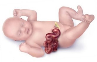
Gastroschisis is a congenital defect of the abdominal wall that leaves a portion of the baby's intestines protruding out of the defect adjacent to the umbilicus.
A number of studies have found evidence that maternal smoking during pregnancy increases the risk of various birth defects in their babies, including gastroschisis. Others have suggested that gastroschisis is more likely with advanced maternal age. Suppose we want to evaluate these risk factors while adjusting for confounding. How can we do this if the outcome variable is dichotomous, not continuous?
To illustrate, suppose we had a large sample and we grouped the mothers by maternal age and looked at the odds that their children would be born with gastroschisis in each group. [This data is hypothetical.] Remember that the odds of an event are:
Odds = P/(1-P)
where P = probability of an event occurring, and (1-P)= probability of the event not occurring.
We are taking a dichotomous outcome that either occurred or didn't occur and expressing it as the odds, i.e., as a continuously distributed outcome. This will tend to create a curvilinear relationship as shown below.
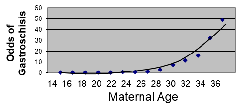
However, if we transform this by taking the log(odds of gastroschisis), it will make this fairly linear.
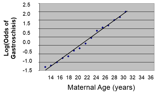
We could describe this relationship in much the same way that we did for simple linear regression, except that the dependent variable is the log(odds of the outcome):
log(Odds of gastrochisis) = b0 + b1(Age)
Therefore, using the log(odds of outcome) as the dependent variable provides a linear relationship that enables us to deal with confounding factors just as we did using multiple linear regression. We previously saw that simple linear regression can be extended to multiple linear regression by adding additional independent variables to the right side of the equation, and the same thing can be done in multiple logistic regression.
A logistic function for health outcomes that occurred or did not occur takes the form shown below.


Where "P" is the probability of the outcome occurring and "(1-P)" is the probability of the event not occurring. Therefore, log[P/(1-P)] is the odds of the outcome occurring.
This is very similar to the form of the multiple linear regression equation except that the dependent variable is an event that occurred or did not occur, and it has been transformed to a continuous variable, i.e., the log(odds of the event occurring). Just as with multiple linear regression, the independent predictor variables can be a mix of continuous, dichotomous, or dummy variables (ordinal or categorical).
Let's start with a simple logistic regression in which we examine the association between maternal smoking during pregnancy and risk of gastroschisis in the offspring, and we can use R to estimate the intercept and slope in the logistic model.
Predictor b p-value OR (95% Conf. Int. for OR)
Intercept -1.052 0.0994
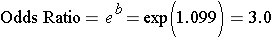
Smoke 1.099 0.2973 3.00 (0.38, 23.68)
As with linear regression, the focus is on the slope, which reflects the association between smoking and the probability of a birth defect). The slope coefficient is 1.099, but remember that we took the log(odds of outcome), so we have to exponentiate the slope coefficient to get the odds ratio.
Here OR=3, meaning that smokers have 3 times the odds of having a baby with birth defects as compared to non-smokers over the study period. The 95% confidence interval for the OR is (0.38, 23.68), so smoking is not statistically significant, because an odds ratio of 1 (the null value here) is included inside the 95% confidence interval.
If you reflect on this, you will realize that this simple logistic regression is looking at the association between a dichotomous outcome (gastroschisis: yes or no) and a dichotomous exposure (smoked during pregnancy: yes or no). This is very much the same as looking at a two by two contingency table and using a chi-squared analysis to evaluate random error.
| Gastroschisis | Normal | |
| Mom Smoked | a | b |
| No Smoke | c | d |
In fact, a chi-squared analysis will give us the same odds ratio and p-value as the simple logistic regression, because smoking is the only independent variable. This simple logistic regression and the chi-square analysis are crude analyses that do not adjust for any confounding factors.
However, we can conduct a multiple logistic regression that simultaneously evaluates the association between gastroschisis and maternal smoking and maternal age.
Predictor b p-value OR (95% Conf. Int. for OR)
Intercept -1.099 0.0994
Smoke 1.062 0.3485 2.89 (0.34, 22.51)
Age 0.298 0.0420 1.35 (1.02, 1.78)
Interpretation:
After controlling for maternal age, mothers who smoked during pregnancy had 2.89 times the odds of giving birth to a child with gastroschisis compared to mothers who did not smoke during pregnancy. And, after controlling for smoking, the odds of delivering a child with gastroschisis were 35% higher for each additional year of maternal age.
Note that this analysis suggests that maternal age is a statistically significant predictor, since the 95% confidence interval does not include the null value. However, after controlling for maternal age, smoking is still not a statistically significant predictor.
 Test Yourself
Researchers wanted to use data collected from a prospective cohort study to develop a model to predict the likelihood of developing hypertension based on age, sex, and body mass index. They performed a multiple logistic regression that gave the following output:
Predictor b p-value OR (95% Conf. Int for OR)
Intercept -5.407 0.0001
Age 0.052 0.0001 1.053 (1.044-1.062)
Male -0.250 0.0007 0.779 (0.674-0.900)
BMI 0.158 0.0001 1.171 (1.146-1.198)
How would you interpret the results for age, sex, and BMI in a few sentences?
Test Yourself
Researchers wanted to use data collected from a prospective cohort study to develop a model to predict the likelihood of developing hypertension based on age, sex, and body mass index. They performed a multiple logistic regression that gave the following output:
Predictor b p-value OR (95% Conf. Int. for OR)
Intercept -5.407 0.0001
Age 0.052 0.0001 1.053 (1.044-1.062)
Male -0.250 0.0007 0.779 (0.674-0.900)
BMI 0.158 0.0001 1.171 (1.146-1.198)
How would you interpret the results for age, sex, and BMI in a few sentences?
Test Yourself
A survey of nursing homes was conducted in 2004 to determine whether there were racial disparities in being vaccinated for influenza. [Li Y and Mukamel D: Racial disparities in receipt of influenza and pneumococcus vaccinations among US nursing home residents. Am J Public Health. 2010l;100(Suppl 1): S256–S262.]
Note that the outcome that the authors reported was not receiving the vaccine.
How would you describe the following results in a few sentences?
|
|
Odds Ratio |
p-value |
|
Black vs. white |
1.84 |
<0.001 |
|
Age (years) <65 65-84 85+ (reference) |
1.30 1.02 1.00 |
0.04 0.811 - |
|
Female gender |
0.97 |
0.76 |
|
Veteran |
0.72 |
0.055 |
|
Length of stay > 6 months |
0.24 |
<0.001 |
|
Heart disease |
0.84 |
0.05 |
|
Chronic pulmonary disease |
1.12 |
0.29 |
|
Asthma |
1.04 |
0.875 |
|
Diabetes |
1.23 |
0.025 |
|
For-profit facility |
1.40 |
0.008 |
|
No. of beds <50 (reference) 50-99 100-199 200+ |
1.00 1.59 1.72 1.87 |
- 0.058 0.024 0.028 |