


Review of Simple Linear Regression
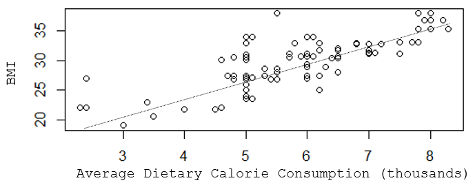
Suppose you wanted to understand the determinants of having a high body mass index (BMI). In this hypothetical example you might find that a scatter plot suggests that there is a reasonably linear association between average dietary caloric intake and BMI, but the R-squared value indicates that caloric intake only explains about two thirds of the variability in BMI.
[NOTE: This is a hypothetical example in which the data was made up to illustrate the teaching points, so the R-squared here is very high, much higher than we generally see in public health data. For example, with coronary artery disease, which has been studied for decades, and for which we know many risk factors, models with all of the known determinants only produce R-squared values of 0.5-0.6.]
> summary(lm(bmi~kcal))
Call:
lm(formula = bmi ~ kcalx1000)
Residuals:
Min 1Q Median 3Q Max
-5.4471 -1.6491 -0.3418 1.3200 9.4227
Coefficients:
Estimate Std. Error t value Pr(>|t|)
(Intercept) 13.8863 1.0635 13.06 <2e-16 ***
Kcal 2.6711 0.1802 14.83 <2e-16 ***
---
Signif. codes: 0 '***' 0.001 '**' 0.01 '*' 0.05 '.' 0.1 ' ' 1
Residual standard error: 2.675 on 109 degrees of freedom
Multiple R-squared: 0.6685, Adjusted R-squared: 0.6655
F-statistic: 219.8 on 1 and 109 DF, p-value: < 2.2e-16
The slope for "kcal" is 2.67, and its standard error is 0.1802, so we can calculate the 95% confidence limit for the slope as follows:
95% confidence interval = Estimate + tcritSE (df=n-2=109)
For 109 degrees of freedom, tcrit = 1.984. Therefore, for kcal the 95% confidence interval = 2.6711 + 1.984 x 0.1802 = (2.31 , 3.03)
Interpretation:
The estimated slope is 2.67 with a margin of error of 0.36. We are 95% confident that the true slope is between 2.31 and 3.03. A slope of 2.67 suggests that each additional 1000 calories in one's daily diet is associated with an increase in BMI of about 2.67 units on average. The confidence interval does not include the null value of 0, so the slope is a statistically significant predictor of BMI at α= 0.05.
While calorie consumption is significant, there are obviously other determinants of BMI, such as age, physical activity, gender, etc. that are other predictors and also potential confounders, meaning that the slope that we obtained for calorie consumption and BMI might not be correct. We need a way to identify multiple determinants of BMI and to evaluate the independent effect of each after controlling for confounding by other determinants.
BMI tends to increase with age, and it may be that some of the variability seen in the previous scatter plot was due to differences in age. I can take age into account if I create a 3-dimensional plot with increasing age projecting back away from me.
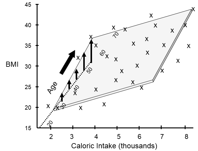
This shows that many of my data points lie close to a plane. The figure above shows the view from the front, and the next image shows a view of the same graph rotated 90 degrees counterclockwise to show the side view.
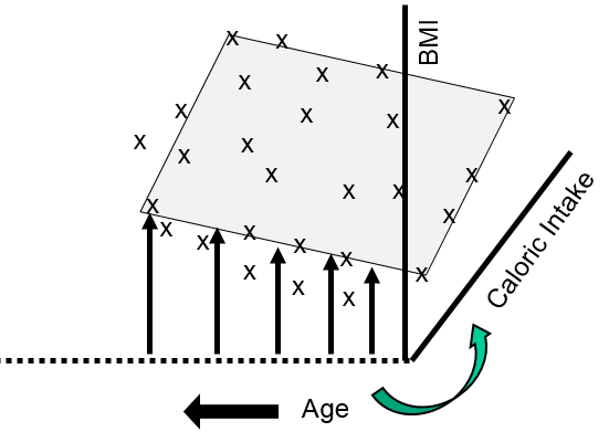
The side view more clearly shows that as age increases there is a tendency for BMI to increase at any given level of caloric intake. We can use multiple linear regression to describe these relationships with an equation and to evaluate the independent effects of calorie consumption and age on BMI as described in the next section.