


Evaluating an Occupational Exposure
An occupational exposure was suspected of damaging lung function and contributing to development of emphysema. The degree of respiratory disability was measured by a technique called spirometry, which is shown below.
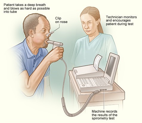
The patient is instructed to breath in and out through a tube connected to a device that records changes in volume. The subject is then instructed to inspire as deeply as possible and then expire as quickly, as forcefully, and as completely as possible. This allows computation of FEV1, the "forced expiratory volume" that can be exhaled in one second. The tracings below are from a normal person and patient with emphysema. Emphysema is a type of chronic obstructive pulmonary disease (COPD). Due to chronic inflammation in the airways, destruction of air sacs, and loss of lung elasticity, the ability to exhale is diminished, and the expiratory phase of breathing is prolonged as shown below.
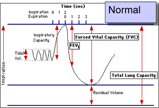
In the normal subject on the left the tracing shows a brisk decrease in volume during forced expiration and a substantial decrease in volume after one second (FEV1).
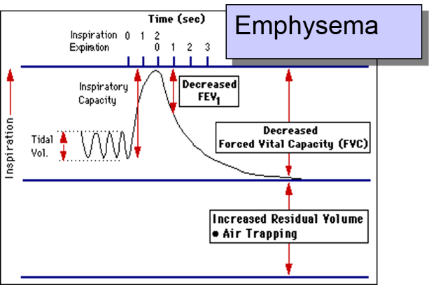
In contrast, when the FEV1 is measured in the patient with emphysema as shown on the right, expiration is greatly delayed and the FEV1 is much smaller. The investigators had subjects who had a potentially harmful occupational exposure and subjects who had not been exposed, and they compared the mean FEV1 in the two groups using a two sample t-test for independent groups. Here are the results:
>t.test(FEV1~Exposure, var.equal=TRUE)
Two Sample t-test
Data: FEV1 by Exposure T = 1.8791, df = 33, p-value = 0.06909
Alternative hypothesis: true difference in means is not equal to 0
95 percent confidence interval:
-0.03653697 0.91987030
Sample estimates
Mean in group 0 mean in group 1
3.895000 3.453333
The difference in means = 3.895-3.453 = 0.4417 liters, which is of borderline statistical significance, since the p-value = 0.069.
Another way of looking at the same question would be to conduct a simple linear regression:
> summary(lm(formula=FEV1~Exposure))
Call:
lm(formula = FEV1 ~ Exposure)
Residuals:
Min 1Q Median 3Q Max
-0.9950 -0.4533 -0.2950 0.5467 1.5467
Coefficients:
Estimate Std. Error t value Pr(>|t)
(Intercept) 3.8950 0.1539 25.313 <2e-16 ***
Exposure -0.4417 0.2350 -1.879 0.0691
--- Signif. Codes: 0 '***' 0.001 '**' '0.01' '*' 0.05 '.' 0.1 ' ' 1
Residual standard error: 0.6881 on 33 degrees of freedom
Multiple R-squared: 0.09666, Adjusted R-squared: 0.06928
F-statistic: 3.531 on 1 an 22 DF, p-value: 0.06909
In the simple linear regression the coefficient for "Exposure" is -0.4417, i.e., the same at the difference in means from the two-sample t-test. This makes sense, because the equation for the regression would be:
FEV1=3.8950 – 0.4417(Exposure)
so, people in the exposed group would be expected to have an FEV1 that was 0.4417 liters less than the unexposed subjects on average. In addition, the p-value for the linear regression is the same as that obtained with the t-test. The point is that the two statistical tests are giving us the same answer.
FEV1 is a sensitive indicator of respiratory impairment, but FEV1 is also known to vary with an individual's height. In other words, height is a confounding variable. What if the exposed and unexposed groups differed in their distribution of height?
The investigators dealt with this by analyzing the data with multiple linear regression as follows:
> summary(lm(FEV1~Exposure + Heightcm))
Call: lm(FEV1=Exposure + Heightcm)
Residuals:
Min 1Q Median 3Q Max
-1.0880 -0.4004 -0.1782 0.3623 1.5224
Coefficients:
Estimate Std. Error t value Pr(.|t|)
(Intercept) -8.87541 3.92911 -2.259 0.0308 *
Exposure -0.53756 0.20902 -2.572 0.0150 *
Heightcm 0.07283 0.02239 3.252 0.0027 **
---
Signif. Codes: 0 '***' 0.001 '**' 0.01 '*' 0.05 '.' 0.1 ' ' 1
Residual standard error: 0.6058 on 32 degrees of freedom
Multiple R-squared: 0.3211, Adjusted R-squared: 0.2786
F-statistic: 7.566 pm 2 and 32 DF, p-value: 0.002039
Interpretation:
Height and "Exposure" are both independent predictors of FEV1. Exposure reduces FEV1 by 0.54 liters after adjusting for differences in height (p-0.015). Exposure and height explain about 32.1% of the variability in FEV1 (p=0.002).
Was there confounding by height?
Here, the measure of effect is the slope. The crude analysis suggested that exposure reduced FEV1 by 0.44 liters, but after adjusting for height, it appears that exposure reduces FEV1 by 0.54 liters.


So, yes, the effect of exposure was confounded by differences in height because the adjusted measure differed from the crude (unadjusted) measure by more than 10%.