PH717 Module 12 - Multiple Variable Regression
Link to video transcript in a Word file
Most health outcomes are multifactorial, meaning that there are multiple factors that influence whether a given outcome will occur, and these other risk factors can introduce confounding that distorts our primary analysis. While stratification is very useful for adjusting for confound by one or two confounders at a time, it is not an efficient way to adjust for multiple confounding factors in a single analysis. In this module we will first extend our discussion of simple linear regression to introduce you to multiple linear regression in which we evaluate multiple independent variables when looking at a continuously distributed dependent variable (health outcome.) We will then introduce multiple logistic regression analysis as a tool for evaluating associations between exposures and dichotomous outcomes. We will draw on examples from the public health literature to discuss the interpretation of results from multiple linear and logistic regression models. You will also gain skills in using R to conduct and interpret these analyses using a public health data set.
Essential Questions
After completing this section, you will be able to:
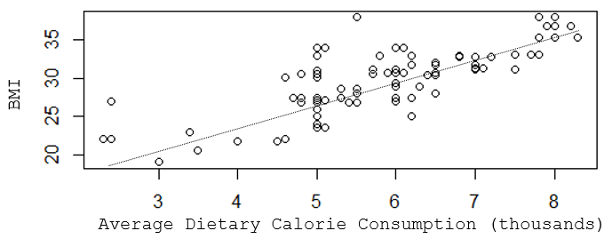
Suppose you wanted to understand the determinants of having a high body mass index (BMI). In this hypothetical example you might find that a scatter plot suggests that there is a reasonably linear association between average dietary caloric intake and BMI, but the R-squared value indicates that caloric intake only explains about two thirds of the variability in BMI.
[NOTE: This is a hypothetical example in which the data was made up to illustrate the teaching points, so the R-squared here is very high, much higher than we generally see in public health data. For example, with coronary artery disease, which has been studied for decades, and for which we know many risk factors, models with all of the known determinants only produce R-squared values of 0.5-0.6.]
> summary(lm(bmi~kcal))
Call:
lm(formula = bmi ~ kcalx1000)
Residuals:
Min 1Q Median 3Q Max
-5.4471 -1.6491 -0.3418 1.3200 9.4227
Coefficients:
Estimate Std. Error t value Pr(>|t|)
(Intercept) 13.8863 1.0635 13.06 <2e-16 ***
Kcal 2.6711 0.1802 14.83 <2e-16 ***
---
Signif. codes: 0 '***' 0.001 '**' 0.01 '*' 0.05 '.' 0.1 ' ' 1
Residual standard error: 2.675 on 109 degrees of freedom
Multiple R-squared: 0.6685, Adjusted R-squared: 0.6655
F-statistic: 219.8 on 1 and 109 DF, p-value: < 2.2e-16
The slope for "kcal" is 2.67, and its standard error is 0.1802, so we can calculate the 95% confidence limit for the slope as follows:
95% confidence interval = Estimate + tcritSE (df=n-2=109)
For 109 degrees of freedom, tcrit = 1.984. Therefore, for kcal the 95% confidence interval = 2.6711 + 1.984 x 0.1802 = (2.31 , 3.03)
Interpretation:
The estimated slope is 2.67 with a margin of error of 0.36. We are 95% confident that the true slope is between 2.31 and 3.03. A slope of 2.67 suggests that each additional 1000 calories in one's daily diet is associated with an increase in BMI of about 2.67 units on average. The confidence interval does not include the null value of 0, so the slope is a statistically significant predictor of BMI at α= 0.05.
While calorie consumption is significant, there are obviously other determinants of BMI, such as age, physical activity, gender, etc. that are other predictors and also potential confounders, meaning that the slope that we obtained for calorie consumption and BMI might not be correct. We need a way to identify multiple determinants of BMI and to evaluate the independent effect of each after controlling for confounding by other determinants.
BMI tends to increase with age, and it may be that some of the variability seen in the previous scatter plot was due to differences in age. I can take age into account if I create a 3-dimensional plot with increasing age projecting back away from me.
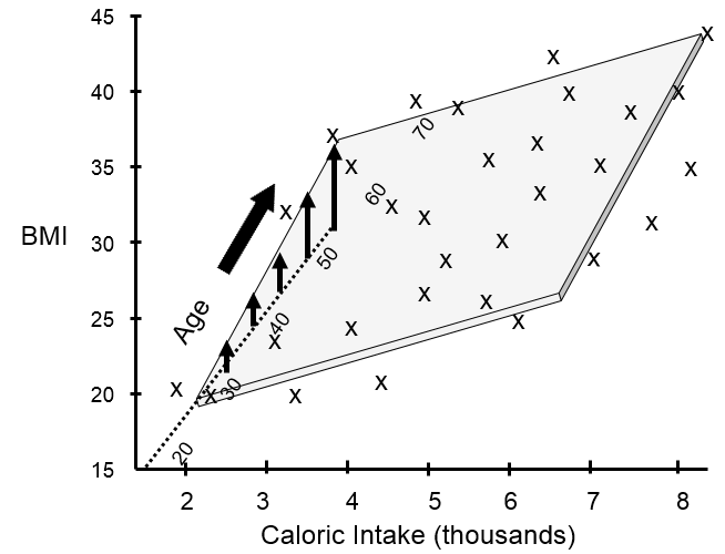
This shows that many of my data points lie close to a plane. The figure above shows the view from the front, and the next image shows a view of the same graph rotated 90 degrees counterclockwise to show the side view.
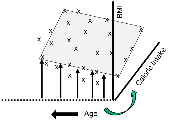
The side view more clearly shows that as age increases there is a tendency for BMI to increase at any given level of caloric intake. We can use multiple linear regression to describe these relationships with an equation and to evaluate the independent effects of calorie consumption and age on BMI as described in the next section.
Multiple linear regression is an extension of simple linear regression that allows us to take into account the effects of other independent predictors (risk factors) on the outcome of interest. And as with simple linear regression, the regression can be summarized with a mathematical equation. An equation for multiple linear regression has the general form shown below.
Y = b0 + b1X1 + b2X2 + b3X3 .. bnXn
Where Y is a continuous measurement outcome (e.g., BMI), b0 is the "intercept" or starting value. X1, X2, X3, etc. are the values of independent predictor variables (i.e., risk factors), and b1, b2, b3, etc. are the coefficients for each risk factor.
Several things are noteworthy:
Adding a Second Predictor Variable
Here is the code and resulting output for the example above looking at the effects of calorie consumption and age on BMI:
> summary(lm(bmi~kcal+age))
Call:
lm(formula = bmi ~ cal + age)
Residuals:
Min 1Q Median 3Q Max
-5.1902 -1.1148 -0.3207 0.9346 6.5912
Coefficients:
Estimate Std. Error t value Pr(>|t|)
(Intercept) 10.50731 0.94086 11.17 < 2e-16 ***
cal 2.43710 0.14572 16.73 < 2e-16 ***
age 0.10711 0.01324 8.09 9.51e-13 ***
---
Signif. codes: 0 '***' 0.001 '**' 0.01 '*' 0.05 '.' 0.1 ' ' 1
Residual standard error: 2.121 on 108 degrees of freedom
Multiple R-squared: 0.7936, Adjusted R-squared: 0.7898
F-statistic: 207.6 on 2 and 108 DF, p-value: < 2.2e-16
The section called "Coefficients" shows Estimate (i.e., the coefficient) for the intercept and for each of the two independent predictors (Kcal and age). The last column shows the p-values for each independent variable, and, in this case, they are both statistically significant independent predictors of BMI. In addition, the p-value at the end of the last line of output is the p-value for the model overall, and that is highly significant also.
Also, notice that the Multiple R-squared is now 0.7936, suggesting that 79% of the variability in BMI can be explained by differences in calorie consumption and age.
In this case, the intercept is not interpretable, but would be included in an equation summarizing these relationships:
BMI = 10.51 + 2.44(cal) + 0.11(age)
This predicts, for example, that a 50 year old who consumes 3000 calories per day on average would have a BMI=34.3. In contrast, a 50 year old consuming 2000 calories per day on average would be predicted to have a BMI=28.2.
By including the age variable in this mathematical model, the coefficient for calories (kcal) is adjusted for confounding by age. Note that the coefficient for kcal is now different from that obtained previously with simple linear regression. We can determine if there was confounding by age by determining if the coefficient for kcal has changed by 10% or more:

It is very close to 10% suggesting that there was perhaps some confounding by age.
Adding a Third Predictor Variable
Now let's add a variable for physical activity to the regression model. Let's assume that I have recorded a variable called "activity" that estimates each subject's weekly Met-hours, a validated way of summarizing their overall activity, and I have assigned each subject to one of three activity levels based on their Met-hours per week.
If I were to try to visualize the combined effects of calorie consumption, age, and level of physical activity in a single graph, it might look something like this:
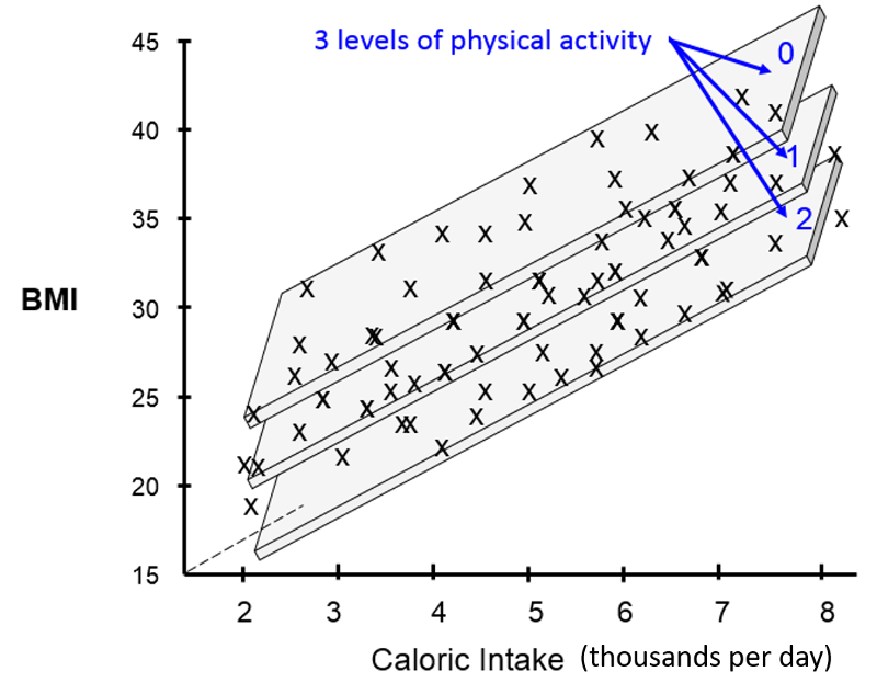
[Note that these illustrations would not be included in a scientific report or publication. I have created these using an artificial data set in order to help you develop an intuitive sense of what we are trying to describe and evaluate with multiple linear regression.]
The illustration above provides a 3-dimensional representation of the impact of all three independent predictor variables on BMI. The Y-axis is still the dependent variable, BMI. The X-axis still represents average daily calorie consumption, and the Z-axis (the dotted line projecting away from us) still represents increasing age. The impact of the three activity levels is shown by the fact that we now have three parallel planes suspended in this three dimensional space, one for each level of physical activity, with the plane for the least active at the top (less active people have higher BMIs) and the most active at the bottom (more active people have lower BMIs).
If we conducted a multiple linear regression analysis of these data using R, the coding and output might look like the following:
> summary(lm(bmi~cal+age+activity))
Call: lm(formula = bmi ~ cal + age + activity)
Residuals:
Min 1Q Median 3Q Max
-6.0253 -0.6509 -0.2472 0.2386 6.1955
Coefficients: Estimate Std. Error t value Pr(>|t|)
(Intercept) 15.47210 1.31819 11.737 < 2e-16 ***
cal 2.00612 0.15831 12.672 < 2e-16 ***
age 0.11146 0.01203 9.262 2.39e-15 ***
activity -1.34302 0.27187 -4.940 2.90e-06 ***
---
Signif. codes: 0 '***' 0.001 '**' 0.01 '*' 0.05 '.' 0.1 ' ' 1
Residual standard error: 1.923 on 107 degrees of freedom Multiple R-squared: 0.8319, Adjusted R-squared: 0.8272
F-statistic: 176.5 on 3 and 107 DF, p-value: < 2.2e-16
We have now accounted for even more of the variability in BMI, since the multiple R-squared has now increased to 0.83. The coefficients for kcal and age have changed slightly after adjusting for confounding by activity level. We can see that shifting from activity level 0 to activity level 1 is associated with a decrease in BMI of 1.34 units on average. Increasing from activity level 2 to activity level 3 would be associated with an additional decrease of 1.34 BMI units.
The coefficients in the analysis show the independent effect of each of these three factors after adjusting for confounding by the other two factors. In other words, the coefficient for average daily calorie intake is adjusted to account for differences in age and activity, and the coefficient for activity level is adjusted to account for differences in age and calorie intake.
Coefficients:
Estimate Std. Error t value Pr(>|t|)
(Intercept) 15.47210 1.31819 11.737 < 2e-16 ***
cal 2.00612 0.15831 12.672 < 2e-16 ***
age 0.11146 0.01203 9.262 2.39e-15 ***
activity -1.34302 0.27187 -4.940 2.90e-06 ***
An Independent Effect
In order to clearly understand what is meant by the coefficients in a multiple linear regression equation, i.e., their independent effect, consider the following hypothetical example looking at the relationship between average daily calorie consumption and BMI in a different population.
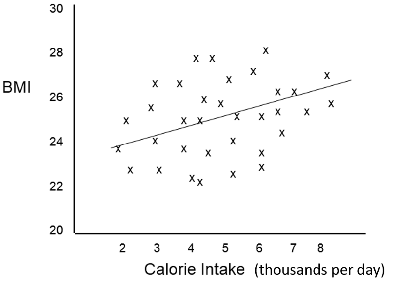
The scatter plot suggests that caloric intake by itself does not predict BMI accurately, and the Multiple R=squared in a simple linear regression was only 0.12. However, the investigators were aware that the effect of caloric intake might be masked due to confounding by other factors such as age and sex, and a multiple linear regression analysis was done revealing that the scatter plot contained four distinct subgroups based on sex and physical activity and that, if differences in activity and sex were taken into account, calorie intake was actually a significant predictor of BMI.

The multiple linear regression analysis provided coefficients for the following equation:
BMI = 15.0 + 1.5 (cal) + 1.6 (if male) - 4.2 (if active)
And the multiple R-squared=0.89
The graph allows us to clearly see what the coefficients are telling us. Suppose we "control for" caloric intake by just focusing on a specific calorie intake, say 5000 calories per day, and also "control" for activity by focusing on activity level 1. If we focus on people with 5000 calorie intakes and activity levels of 1, the effect of being a male compared to a female is an increase of 1.6 units in predicted BMI.
Similarly, if we focus on females with 5000 calorie intakes, the effect of moving from an active female to an inactive female is a predicted increase of 4.2 units in BMI. Finally, at any of the four categories of sex and activity the slope of the line for the effect of caloric intake is 1.5. Thus, the coefficients indicate the incremental change in the dependent variable for each increment in any of the independent variables after controlling for the other variables in the model.
 Test Yourself
Suppose we had observed the following relationship between caloric intake and BMI in inactive males and females. What phenomenon does this depict?
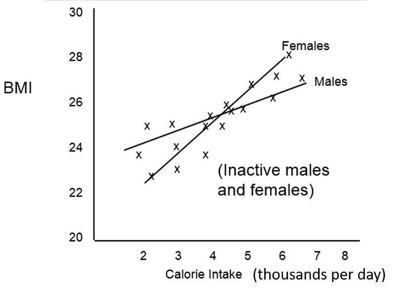
Answer
An occupational exposure was suspected of damaging lung function and contributing to development of emphysema. The degree of respiratory disability was measured by a technique called spirometry, which is shown below.
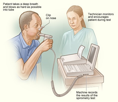
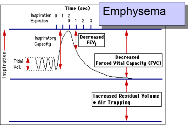
The patient is instructed to breath in and out through a tube connected to a device that records changes in volume. The subject is then instructed to inspire as deeply as possible and then expire as quickly, as forcefully, and as completely as possible. This allows computation of FEV1, the "forced expiratory volume" that can be exhaled in one second. The tracings below are from a normal person and patient with emphysema. Emphysema is a type of chronic obstructive pulmonary disease (COPD). Due to chronic inflammation in the airways, destruction of air sacs, and loss of lung elasticity, the ability to exhale is diminished, and the expiratory phase of breathing is prolonged as shown below.
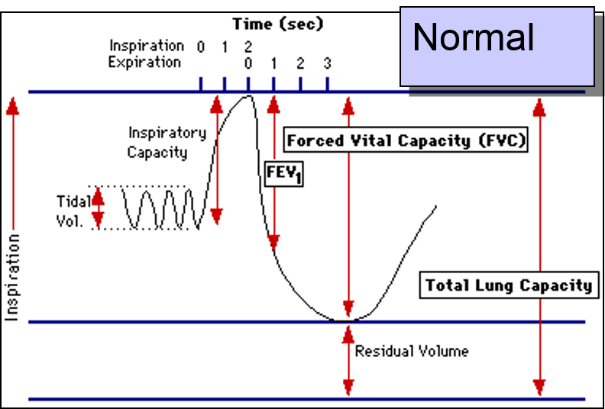
In the normal subject on the left the tracing shows a brisk decrease in volume during forced expiration and a substantial decrease in volume after one second (FEV1).
In contrast, when the FEV1 is measured in the patient with emphysema as shown on the right, expiration is greatly delayed and the FEV1 is much smaller. The investigators had subjects who had a potentially harmful occupational exposure and subjects who had not been exposed, and they compared the mean FEV1 in the two groups using a two sample t-test for independent groups. Here are the results:
>t.test(FEV1~Exposure, var.equal=TRUE)
Two Sample t-test
Data: FEV1 by Exposure T = 1.8791, df = 33, p-value = 0.06909
Alternative hypothesis: true difference in means is not equal to 0
95 percent confidence interval:
-0.03653697 0.91987030
Sample estimates
Mean in group 0 mean in group 1
3.895000 3.453333
The difference in means = 3.895-3.453 = 0.4417 liters, which is of borderline statistical significance, since the p-value = 0.069.
Another way of looking at the same question would be to conduct a simple linear regression:
> summary(lm(formula=FEV1~Exposure))
Call:
lm(formula = FEV1 ~ Exposure)
Residuals:
Min 1Q Median 3Q Max
-0.9950 -0.4533 -0.2950 0.5467 1.5467
Coefficients:
Estimate Std. Error t value Pr(>|t)
(Intercept) 3.8950 0.1539 25.313 <2e-16 ***
Exposure -0.4417 0.2350 -1.879 0.0691
--- Signif. Codes: 0 '***' 0.001 '**' '0.01' '*' 0.05 '.' 0.1 ' ' 1
Residual standard error: 0.6881 on 33 degrees of freedom
Multiple R-squared: 0.09666, Adjusted R-squared: 0.06928
F-statistic: 3.531 on 1 an 22 DF, p-value: 0.06909
In the simple linear regression the coefficient for "Exposure" is -0.4417, i.e., the same at the difference in means from the two-sample t-test. This makes sense, because the equation for the regression would be:
FEV1=3.8950 – 0.4417(Exposure)
so, people in the exposed group would be expected to have an FEV1 that was 0.4417 liters less than the unexposed subjects on average. In addition, the p-value for the linear regression is the same as that obtained with the t-test. The point is that the two statistical tests are giving us the same answer.
FEV1 is a sensitive indicator of respiratory impairment, but FEV1 is also known to vary with an individual's height. In other words, height is a confounding variable. What if the exposed and unexposed groups differed in their distribution of height?
The investigators dealt with this by analyzing the data with multiple linear regression as follows:
> summary(lm(FEV1~Exposure + Heightcm))
Call: lm(FEV1=Exposure + Heightcm)
Residuals:
Min 1Q Median 3Q Max
-1.0880 -0.4004 -0.1782 0.3623 1.5224
Coefficients:
Estimate Std. Error t value Pr(.|t|)
(Intercept) -8.87541 3.92911 -2.259 0.0308 *
Exposure -0.53756 0.20902 -2.572 0.0150 *
Heightcm 0.07283 0.02239 3.252 0.0027 **
---
Signif. Codes: 0 '***' 0.001 '**' 0.01 '*' 0.05 '.' 0.1 ' ' 1
Residual standard error: 0.6058 on 32 degrees of freedom
Multiple R-squared: 0.3211, Adjusted R-squared: 0.2786
F-statistic: 7.566 pm 2 and 32 DF, p-value: 0.002039
Interpretation:
Height and "Exposure" are both independent predictors of FEV1. Exposure reduces FEV1 by 0.54 liters after adjusting for differences in height (p-0.015). Exposure and height explain about 32.1% of the variability in FEV1 (p=0.002).
Was there confounding by height?
Here, the measure of effect is the slope. The crude analysis suggested that exposure reduced FEV1 by 0.44 liters, but after adjusting for height, it appears that exposure reduces FEV1 by 0.54 liters.

So, yes, the effect of exposure was confounded by differences in height because the adjusted measure differed from the crude (unadjusted) measure by more than 10%.
In regression analyses, categorical predictors are represented using 0 and 1 for dichotomous variables or using indicator (or dummy) variables for ordinal or categorical variables.
Suppose we wanted to conduct an analysis to determine whether systolic blood pressure is lower in people who exercise regularly compared to people who don't after adjusting for AGE (in years), use of blood pressure lowering medications (BPMEDS), and BMI. However, instead of treating BMI as a continuous variable, we want to collapse BMI into four categories (underweight, normal, overweight, & obese).
I want to make the "normal" BMI category the reference, so I need to make indicator variables for being underweight, overweight, or obese. To do this in R, we can use ifelse() statements to create the indicator variables. The general form of an ifelse() statement is:
(new_variable_name)<-ifelse(conditional_test, value_assigned_if true, value_assigned_if_not_true)
For example, I can create new dummy variables to create indicators for the underweight, overweight, and obese BMI categories as follows:
> underwgt<-ifelse(BMI<18.5, 1, 0)
> overwgt<-ifelse(BMI>=25 & BMI<30, 1, 0)
> obese<-ifelse(BMI>=30, 1, 0)
The first command above evaluates each subject's BMI, and if it is less than 18.5, it assigns a value of 1 to a new variable called "underwgt"; if BMI is not less than 18.5, R assigns a value of 0 to "underwgt". Similarly, the seconde command creates a new variable called "overwgt" and assigns it a value of 1 if BMI is greater than 25 and less than 30, and it assigns a value of 0 if BMI is either below or above this range. Finally, the third command creates a variable called "obese" which has a value of 1 of BMI is greater than or equal to 30, and has a value of 0 if BMI is less than 30.
Note that I don't need to include a statement to define "normal" because all the normal subjects (who are not in any of the other three categories) will not have an indicator variable assigned, so they will become the reference group for the other three variables by default. The "ifelse" commands above would assign the values shown in the table below.
|
BMI Categories |
Underweight |
Normal |
Overweight |
Obese |
|
underwgt |
1 |
0 |
0 |
0 |
|
overwgt |
0 |
0 |
1 |
0 |
|
obese |
0 |
0 |
0 |
1 |
Once the dummy variables have been created, we can perform a multiple linear regression that includes this set of indicators in addition to other independent variables. Note that BPMEDS is a dichotomous variable coded 1 if any BP medications are used and coded 0 if not. The variable MALE was coded 1 for males and 0 for females. To perform this regression analysis in R, we use the following code:
> lm3<-lm(SYSBP~underwgt+overwgt+obese+AGE+MALE+BPMEDS)
> summary(lm3)
Call:
lm(formula = SYSBP ~ underwgt + overwgt + obese + AGE + MALE + BPMEDS)
Residuals:
Min 1Q Median 3Q Max
-57.521 -12.845 -2.209 9.979 139.606
Coefficients:
Estimate Std. Error t value Pr(>|t|)
(Intercept) 84.67507 1.73970 48.672 < 2e-16 ***
underwgt -6.46970 2.58809 -2.500 0.0125 *
overwgt 7.20117 0.64426 11.177 < 2e-16 ***
obese 14.85372 0.92743 16.016 < 2e-16 ***
AGE 0.87289 0.03431 25.444 < 2e-16 ***
MALE -2.40472 0.59802 -4.021 5.89e-05 ***
BPMEDS 25.02151 1.65839 15.088 < 2e-16 ***
--- Signif. codes: 0 '***' 0.001 '**' 0.01 '*' 0.05 '.' 0.1 ' ' 1
Residual standard error: 19.24 on 4347 degrees of freedom (80 observations deleted due to missingness)
Multiple R-squared: 0.2585, Adjusted R-squared: 0.2574
F-statistic: 252.5 on 6 and 4347 DF, p-value: < 2.2e-16
Interpretation:
The overall p-value for the model on the last row of output indicates that the model is highly significant, so we can interpret the results for individual variables in the model. After controlling for confounding with multiple linear regression, each of these predictor variables has a statistically significant association with systolic blood pressure. Subjects who are underweight have systolic blood pressures that are about 6 mm Hg lower that that in subjects with BMI in the normal range after adjusting for other variables in the model. Those who are overweight have systolic blood pressures that are about 7 mm Hg higher than those of normal individuals, and obese people have systolic blood pressures about 15 mm Hg higher than subjects with a normal BMI. AGE is associated with a small but statistically significant increase in systolic blood pressure, i.e., an increase of just less than 1 mm Hg for each additional year of age. Not surprisingly, those using blood pressure lowering medications had pressures 25 mm Hg lower than those not using such medications. [There is a lot of undiagnosed/untreated high blood pressure in the population.]
Suppose that instead of a continuous variable for BMI, the data set already has a categorical variable called "bmicat" that is coded 1, 2, 3, 4 to indicate those who are underweight, normal weight, overweight, or obese.
In this situation you can use the factor( ) command in R to create dummy variables using a coding statement like the one shown below.
> summary(lm(sysbp ~ age + studygrp + factor(bmicat)))
The factor( ) command makes the lowest coded category the reference unless you specify otherwise. For example, if the data is coded 1, 2, 3, 4, R will use category 1 (underweight subjects) as the reference. However, you can use the relevel( ) command to specify the reference. Here it makes sense to use 'normal weight', i.e., BMIcat = 2, as the reference, as below.
> summary(lm(sysbp~age + studygrp + relevel(factor BMIcat),ref="2")))
This would produce the following output:
Call: lm(formula = sysbp ~ age + studygrp + relevel(factor(BMIcat), ref = "2"))
Coefficients:
Estimate Std. Error t value Pr(>|t|)
(Intercept) 86.3514 6.1109 14.131 < 2e-16 ***
age 0.6676 0.1065 6.266 4.04e-09 ***
studygrp 4.4550 2.6644 1.672 0.09668 .
relevel(factor(BMIcat),ref="2")1 -30.3576 11.0720 -2.742 0.00689 **
relevel(factor(BMIcat),ref="2")3 2.0878 2.6448 0.789 0.43118
relevel(factor(BMIcat),ref="2")4 15.4479 6.0609 2.549 0.01186 *
---
Signif. codes: 0 '***' 0.001 '**' 0.01 '*' 0.05 '.' 0.1 ' ' 1
Residual standard error: 15.29 on 144 degrees of freedom
Multiple R-squared: 0.2884, Adjusted R-squared: 0.2637
F-statistic: 11.67 on 5 and 144 DF, p-value: 1.767e-09
Multiple linear regression is used to evaluate predictors for a continuously distributed outcome variable. The procedure calculates coefficients for each of the independent variables (predictors) that best agree with the observed data in the sample.
Multiple variable regression enables you to:
Interpretation:
Test Yourself
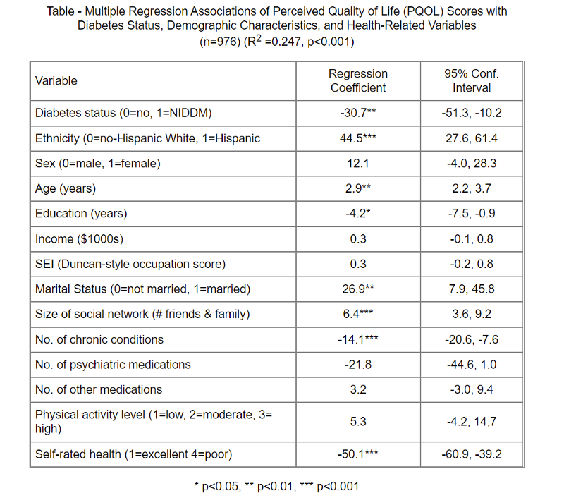
A study was conducted to evaluate the association between quality of life and non-insulin-dependent diabetes mellitus (NIDDM) status, and whether this association differs between Hispanics and non-Hispanic Whites. Between 1986 and 1989, cross-sectional data on perceived quality of life (PQOL) were collected from 223 persons with NIDDM and 753 non-diabetic subjects.
What would you conclude regarding the results of multiple linear regression analysis summarized in the table below? How would you summarize these findings for a general audience? Remember that the regression coefficients can be thought of as slopes with a null value=0.
Table - Multiple Regression Associations of Perceived Quality of Life (PQOL) Scores with
Diabetes Status, Demographic Characteristics, and Health-Related Variables
(n=976) (R2 =0.247, p<0.001)
Answer
Test Yourself
A prospective cohort study was conducted in the women and children's clinic at Boston City Hospital from 1984 to 1987 to determine the effects of maternal use of tobacco, alcohol, marijuana, cocaine, and other drugs during pregnancy. Exposures were assessed during pregnancy in 1,226 women using questionnaires and urine tests for cocaine and marijuana. The primary outcome was birth weight of their baby. [Zuckerman B, et al.: Effects of Maternal Marijuana and Cocaine Use on Fetal Growth, N. Engl. J. Med. 1989; 320:762-768]
A t-test for independent samples found that babies born to mothers who used cocaine during pregnancy weighed on average 407 grams less than babies born to mothers who did not use cocaine. However, mothers who use cocaine during pregnancy differed from non-users in a number of other ways that could cause confounding. Cocaine users were also more likely to smoke cigarettes and drink alcohol during pregnancy, and they were more likely to have sexually transmitted infections during their pregnancy.
The investigators conducted a multiple linear regression with the following results:
Note that the data for gestational age and maternal age were not normally distributed, so the investigators used log transformations to normalize the data.
Variable Coefficient p-value
Gestational age (log) 6452 .001
Maternal age (log) -85 .210
Maternal weight gain (lb.) 7 .001
Hispanic vs Black 106 .004
White vs Black 199 .001
Primipara (1st pregnancy) -141 .001
Number of prenatal visits 16 .001
Cocaine use(1=yes; 0=no) -93 .070
R2 = 0.51
Interpret these results with respect to:
Answer
Test Yourself
A clinical trial was conducted to investigate the efficacy of antenatal corticosteroids in reducing neonatal morbidity in women at risk for preterm delivery.
The primary outcome was a composite including any of the following: respiratory distress syndrome, bronchopulmonary dysplasia, severe intraventricular hemorrhage, sepsis and perinatal death. However, for this exercise we will focus on birth weight, which was one of the continuous outcome outcomes.
The data are posted in a file called "Steroids_rct.csv", which you can download from the data set folder on Blackboard. The variables are named and codes are as follows:
Variable Coded as:
treatment 1=steroids; 0=placebo
malesex 1=male; 0=female
gestage gestational age (in weeks)
birthweight Weight of the infant at birth in grams
mat_age maternal age in years
outcome 1=yes; 0=no
Link to answer in a Word file
The goal of logistic regression is the same as multiple linear regression, but the key difference is that multiple linear regression evaluates predictors of continuously distributed outcomes, while multiple logistic regression evaluates predictors of dichotomous outcomes, i.e., outcomes that either occurred or did not.
Gastroschisis is a congenital defect of the abdominal wall that leaves a portion of the baby's intestines protruding out of the defect adjacent to the umbilicus.
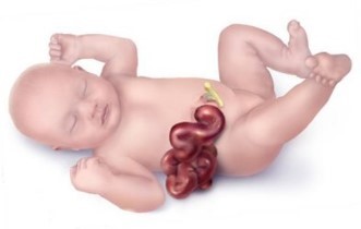
A number of studies have found evidence that maternal smoking during pregnancy increases the risk of various birth defects in their babies, including gastroschisis. Others have suggested that gastroschisis is more likely with advanced maternal age. Suppose we want to evaluate these risk factors while adjusting for confounding. How can we do this if the outcome variable is dichotomous, not continuous?
To illustrate, suppose we had a large sample and we grouped the mothers by maternal age and looked at the odds that their children would be born with gastroschisis in each group. [This data is hypothetical.] Remember that the odds of an event are:
Odds = P/(1-P)
where P = probability of an event occurring, and (1-P)= probability of the event not occurring.
We are taking a dichotomous outcome that either occurred or didn't occur and expressing it as the odds, i.e., as a continuously distributed outcome. This will tend to create a curvilinear relationship as shown below.
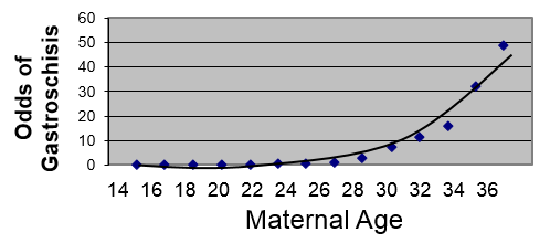
However, if we transform this by taking the log(odds of gastroschisis), it will make this fairly linear.
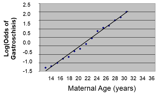
We could describe this relationship in much the same way that we did for simple linear regression, except that the dependent variable is the log(odds of the outcome):
log(Odds of gastrochisis) = b0 + b1(Age)
Therefore, using the log(odds of outcome) as the dependent variable provides a linear relationship that enables us to deal with confounding factors just as we did using multiple linear regression. We previously saw that simple linear regression can be extended to multiple linear regression by adding additional independent variables to the right side of the equation, and the same thing can be done in multiple logistic regression.
A logistic function for health outcomes that occurred or did not occur takes the form shown below.

Where "P" is the probability of the outcome occurring and "(1-P)" is the probability of the event not occurring. Therefore, log[P/(1-P)] is the odds of the outcome occurring.
This is very similar to the form of the multiple linear regression equation except that the dependent variable is an event that occurred or did not occur, and it has been transformed to a continuous variable, i.e., the log(odds of the event occurring). Just as with multiple linear regression, the independent predictor variables can be a mix of continuous, dichotomous, or dummy variables (ordinal or categorical).
Let's start with a simple logistic regression in which we examine the association between maternal smoking during pregnancy and risk of gastroschisis in the offspring, and we can use R to estimate the intercept and slope in the logistic model.
Predictor b p-value OR (95% Conf. Int. for OR)
Intercept -1.052 0.0994
Smoke 1.099 0.2973 3.00 (0.38, 23.68)
As with linear regression, the focus is on the slope, which reflects the association between smoking and the probability of a birth defect). The slope coefficient is 1.099, but remember that we took the log(odds of outcome), so we have to exponentiate the slope coefficient to get the odds ratio.
Here OR=3, meaning that smokers have 3 times the odds of having a baby with birth defects as compared to non-smokers over the study period. The 95% confidence interval for the OR is (0.38, 23.68), so smoking is not statistically significant, because an odds ratio of 1 (the null value here) is included inside the 95% confidence interval.
If you reflect on this, you will realize that this simple logistic regression is looking at the association between a dichotomous outcome (gastroschisis: yes or no) and a dichotomous exposure (smoked during pregnancy: yes or no). This is very much the same as looking at a two by two contingency table and using a chi-squared analysis to evaluate random error.
| Gastroschisis | Normal | |
| Mom Smoked | a | b |
| No Smoke | c | d |
In fact, a chi-squared analysis will give us the same odds ratio and p-value as the simple logistic regression, because smoking is the only independent variable. This simple logistic regression and the chi-square analysis are crude analyses that do not adjust for any confounding factors.
However, we can conduct a multiple logistic regression that simultaneously evaluates the association between gastroschisis and maternal smoking and maternal age.
Predictor b p-value OR (95% Conf. Int. for OR)
Intercept -1.099 0.0994
Smoke 1.062 0.3485 2.89 (0.34, 22.51)
Age 0.298 0.0420 1.35 (1.02, 1.78)
Interpretation:
After controlling for maternal age, mothers who smoked during pregnancy had 2.89 times the odds of giving birth to a child with gastroschisis compared to mothers who did not smoke during pregnancy. And, after controlling for smoking, the odds of delivering a child with gastroschisis were 35% higher for each additional year of maternal age.
Note that this analysis suggests that maternal age is a statistically significant predictor, since the 95% confidence interval does not include the null value. However, after controlling for maternal age, smoking is still not a statistically significant predictor.
Test Yourself
Researchers wanted to use data collected from a prospective cohort study to develop a model to predict the likelihood of developing hypertension based on age, sex, and body mass index. They performed a multiple logistic regression that gave the following output:
Predictor b p-value OR (95% Conf. Int for OR)
Intercept -5.407 0.0001
Age 0.052 0.0001 1.053 (1.044-1.062)
Male -0.250 0.0007 0.779 (0.674-0.900)
BMI 0.158 0.0001 1.171 (1.146-1.198)
How would you interpret the results for age, sex, and BMI in a few sentences?
Answer
Test Yourself
Researchers wanted to use data collected from a prospective cohort study to develop a model to predict the likelihood of developing hypertension based on age, sex, and body mass index. They performed a multiple logistic regression that gave the following output:
Predictor b p-value OR (95% Conf. Int. for OR)
Intercept -5.407 0.0001
Age 0.052 0.0001 1.053 (1.044-1.062)
Male -0.250 0.0007 0.779 (0.674-0.900)
BMI 0.158 0.0001 1.171 (1.146-1.198)
How would you interpret the results for age, sex, and BMI in a few sentences?
Answer
Test Yourself
A survey of nursing homes was conducted in 2004 to determine whether there were racial disparities in being vaccinated for influenza. [Li Y and Mukamel D: Racial disparities in receipt of influenza and pneumococcus vaccinations among US nursing home residents. Am J Public Health. 2010l;100(Suppl 1): S256–S262.]
Note that the outcome that the authors reported was not receiving the vaccine.
How would you describe the following results in a few sentences?
|
|
Odds Ratio |
p-value |
|
Black vs. white |
1.84 |
<0.001 |
|
Age (years) <65 65-84 85+ (reference) |
1.30 1.02 1.00 |
0.04 0.811 - |
|
Female gender |
0.97 |
0.76 |
|
Veteran |
0.72 |
0.055 |
|
Length of stay > 6 months |
0.24 |
<0.001 |
|
Heart disease |
0.84 |
0.05 |
|
Chronic pulmonary disease |
1.12 |
0.29 |
|
Asthma |
1.04 |
0.875 |
|
Diabetes |
1.23 |
0.025 |
|
For-profit facility |
1.40 |
0.008 |
|
No. of beds <50 (reference) 50-99 100-199 200+ |
1.00 1.59 1.72 1.87 |
- 0.058 0.024 0.028 |
Answer
A survey was conducted among 600 teenagers to determine factors related to the likelihood of wearing a seatbelt when in a motor vehicle. The primary outcome was whether a seatbelt was always worn (coded 0 for no and 1 for yes). The independent variables were grade in school (grade), male sex (sexm), Hispanic (0 or 1), Asian (0 or 1), other race (raceother, coded 0 or 1), riding with a drinking driver (ridedd, coded 0 or 1), and having smoked tobacco in the past 30 days (smoke30, coded 0 or 1).
A multiple logistic regression analysis can be performed using the "glm" function in R (general linear models). "glm" includes different procedures so we need to add the code at the end "family=binomial (link=logit)" to indicate logistic regression. We can conduct the logistic analysis using the code below:
>log.out <-glm(beltalways~sexm + grade + hispanic + asian + raceother + ridedd + smoke30, family=binomial (link=logit))
> summary(log.out)
The default output gives the regression slopes which can be used to judge the direction of associations and their statistical significance.
Coefficients: Estimate Std. Error z value Pr(>|z|)
(Intercept) -1.31109 0.84639 -1.549 0.121376
sexm -0.15505 0.17060 -0.909 0.363414
grade 0.17192 0.07599 2.262 0.023672 *
hispanic -0.10128 0.20118 -0.503 0.614646
asian -0.32015 0.30163 -1.061 0.288514
raceother -0.01991 0.42393 -0.047 0.962535
ridedd -0.65090 0.18932 -3.438 0.000586 ***
smoke30 -0.60969 0.24168 -2.523 0.011646
However, since we used log(odds of seatbelt use) as the outcome, we need to exponentiate the coefficients in order to get the odds ratios. R can do this for us with the following command:
> exp(log.out$coeff)
(Intercept) sexm grade hispanic asian raceother
0.2695271 0.8563720 1.1875858 0.9036756 0.7260428 0.9802837
ridedd smoke30
0.5215746 0.5435210
R will also generate the 95% confidence limits for each of these.
> exp(confint(log.out))
Waiting for profiling to be done...
2.5% 97.5%
(Intercept) 0.0510250 1.4138545
sexm 0.6126924 1.1963753
grade 1.0236885 1.3793179
hispanic 0.6086518 1.3404946
asian 0.4010068 1.3119174
raceother 0.4248549 2.2668680
ridedd 0.3590405 0.7547487
smoke30 0.3359862 0.8687327
We might summarize these findings as shown in this table.
| Variable |
Adjusted OR |
95% Confidence Int. |
p-value |
|
Sex (M=1; F=0) |
0.86 |
0.61,1.20 |
0.36 |
|
Grade in School |
1.19 |
1.02, 1.38 |
0.024 |
|
Race/Ethnicity Hispanic vs. white Asian vs. white Other vs. white |
0.90 0.73 0.98 |
0.61, 1.34 0.40, 1.31 0.43, 2.25 |
0.615 0.29 0.963 |
|
Ride with a drinking driver |
0.52 |
0.36, 0.76 |
0.001 |
|
Smoke past 30 days |
0.54 |
0.34, 0.87 |
0.012 |
Test Yourself
Interpret the results of the analysis above in a few sentences. Write down your interpretation before looking at the answer.
Answer
Practice Your R Skills
You previously conducted an analysis of the data set called "Steroids_rct.csv" to determine whether birth weight differed in neonates delivered to mothers who had been treated with steroids. Since birth weight is a continuous outcome, you used multiple linear regression see if there was an association after controlling for confounding.
Recall that the primary outcome was a composite outcome. The outcome variable "outcome" was coded 1 if any one of the designated complications occurred, i.e., respiratory distress syndrome, bronchopulmonary dysplasia, severe intraventricular hemorrhage, sepsis or perinatal death, and "outcome" was coded 0 if none of these occurred. You will now use multiple logistic regression to look at determinants of "outcome."
The data are posted in a file called "Steroids_rct.csv". The variables are named and coded as follows:
|
Variable |
Coded as: |
|
treatment |
1=steroids; 0=placebo |
|
malesex |
1=male; 0=female |
|
gestage |
gestational age in weeks |
|
birthweight |
birthweight of the infant in grams |
|
mat_age |
maternal age in years |
Questions:
Link to answers in a Word file