


Multiple Linear Regression
Multiple linear regression is an extension of simple linear regression that allows us to take into account the effects of other independent predictors (risk factors) on the outcome of interest. And as with simple linear regression, the regression can be summarized with a mathematical equation. An equation for multiple linear regression has the general form shown below.
Y = b0 + b1X1 + b2X2 + b3X3 .. bnXn
Where Y is a continuous measurement outcome (e.g., BMI), b0 is the "intercept" or starting value. X1, X2, X3, etc. are the values of independent predictor variables (i.e., risk factors), and b1, b2, b3, etc. are the coefficients for each risk factor.
Several things are noteworthy:
- Linear regression (both simple and multiple) can be used when the outcome (dependent) variable is continuously distributed, i.e., a measurement variable.
- The independent variables (predictors) can be continuous, dichotomous (yes/no), ordinal, or categorical (dummy variables). Dichotomous variables should be coded as 1 if the factor is true/present and 0 if not. Ordinal and categorical variables (so-called "dummy variables") are coded 1, 2, 3, 4, etc. (discussed in more detail later in this module).
- Note that there can be many more than 3 variables; the total possible number will be limited only by the sample size.
Adding a Second Predictor Variable
Here is the code and resulting output for the example above looking at the effects of calorie consumption and age on BMI:
> summary(lm(bmi~kcal+age))
Call:
lm(formula = bmi ~ cal + age)
Residuals:
Min 1Q Median 3Q Max
-5.1902 -1.1148 -0.3207 0.9346 6.5912
Coefficients:
Estimate Std. Error t value Pr(>|t|)
(Intercept) 10.50731 0.94086 11.17 < 2e-16 ***
cal 2.43710 0.14572 16.73 < 2e-16 ***
age 0.10711 0.01324 8.09 9.51e-13 ***
---
Signif. codes: 0 '***' 0.001 '**' 0.01 '*' 0.05 '.' 0.1 ' ' 1
Residual standard error: 2.121 on 108 degrees of freedom
Multiple R-squared: 0.7936, Adjusted R-squared: 0.7898
F-statistic: 207.6 on 2 and 108 DF, p-value: < 2.2e-16
The section called "Coefficients" shows Estimate (i.e., the coefficient) for the intercept and for each of the two independent predictors (Kcal and age). The last column shows the p-values for each independent variable, and, in this case, they are both statistically significant independent predictors of BMI. In addition, the p-value at the end of the last line of output is the p-value for the model overall, and that is highly significant also.
Also, notice that the Multiple R-squared is now 0.7936, suggesting that 79% of the variability in BMI can be explained by differences in calorie consumption and age.
In this case, the intercept is not interpretable, but would be included in an equation summarizing these relationships:
BMI = 10.51 + 2.44(cal) + 0.11(age)
This predicts, for example, that a 50 year old who consumes 3000 calories per day on average would have a BMI=34.3. In contrast, a 50 year old consuming 2000 calories per day on average would be predicted to have a BMI=28.2.
By including the age variable in this mathematical model, the coefficient for calories (kcal) is adjusted for confounding by age. Note that the coefficient for kcal is now different from that obtained previously with simple linear regression. We can determine if there was confounding by age by determining if the coefficient for kcal has changed by 10% or more:


It is very close to 10% suggesting that there was perhaps some confounding by age.
Adding a Third Predictor Variable
Now let's add a variable for physical activity to the regression model. Let's assume that I have recorded a variable called "activity" that estimates each subject's weekly Met-hours, a validated way of summarizing their overall activity, and I have assigned each subject to one of three activity levels based on their Met-hours per week.
If I were to try to visualize the combined effects of calorie consumption, age, and level of physical activity in a single graph, it might look something like this:
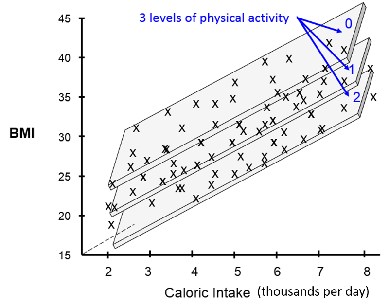
[Note that these illustrations would not be included in a scientific report or publication. I have created these using an artificial data set in order to help you develop an intuitive sense of what we are trying to describe and evaluate with multiple linear regression.]
The illustration above provides a 3-dimensional representation of the impact of all three independent predictor variables on BMI. The Y-axis is still the dependent variable, BMI. The X-axis still represents average daily calorie consumption, and the Z-axis (the dotted line projecting away from us) still represents increasing age. The impact of the three activity levels is shown by the fact that we now have three parallel planes suspended in this three dimensional space, one for each level of physical activity, with the plane for the least active at the top (less active people have higher BMIs) and the most active at the bottom (more active people have lower BMIs).
If we conducted a multiple linear regression analysis of these data using R, the coding and output might look like the following:
> summary(lm(bmi~cal+age+activity))
Call: lm(formula = bmi ~ cal + age + activity)
Residuals:
Min 1Q Median 3Q Max
-6.0253 -0.6509 -0.2472 0.2386 6.1955
Coefficients: Estimate Std. Error t value Pr(>|t|)
(Intercept) 15.47210 1.31819 11.737 < 2e-16 ***
cal 2.00612 0.15831 12.672 < 2e-16 ***
age 0.11146 0.01203 9.262 2.39e-15 ***
activity -1.34302 0.27187 -4.940 2.90e-06 ***
---
Signif. codes: 0 '***' 0.001 '**' 0.01 '*' 0.05 '.' 0.1 ' ' 1
Residual standard error: 1.923 on 107 degrees of freedom Multiple R-squared: 0.8319, Adjusted R-squared: 0.8272
F-statistic: 176.5 on 3 and 107 DF, p-value: < 2.2e-16
We have now accounted for even more of the variability in BMI, since the multiple R-squared has now increased to 0.83. The coefficients for kcal and age have changed slightly after adjusting for confounding by activity level. We can see that shifting from activity level 0 to activity level 1 is associated with a decrease in BMI of 1.34 units on average. Increasing from activity level 2 to activity level 3 would be associated with an additional decrease of 1.34 BMI units.
Independent (Unconfounded) Effects
The coefficients in the analysis show the independent effect of each of these three factors after adjusting for confounding by the other two factors. In other words, the coefficient for average daily calorie intake is adjusted to account for differences in age and activity, and the coefficient for activity level is adjusted to account for differences in age and calorie intake.
Coefficients:
Estimate Std. Error t value Pr(>|t|)
(Intercept) 15.47210 1.31819 11.737 < 2e-16 ***
cal 2.00612 0.15831 12.672 < 2e-16 ***
age 0.11146 0.01203 9.262 2.39e-15 ***
activity -1.34302 0.27187 -4.940 2.90e-06 ***
An Independent Effect
In order to clearly understand what is meant by the coefficients in a multiple linear regression equation, i.e., their independent effect, consider the following hypothetical example looking at the relationship between average daily calorie consumption and BMI in a different population.
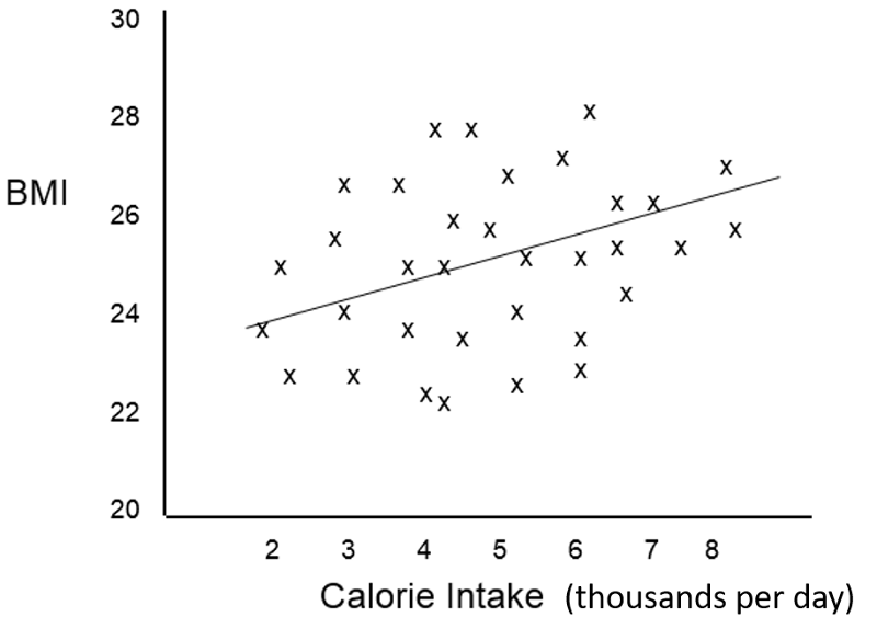
The scatter plot suggests that caloric intake by itself does not predict BMI accurately, and the Multiple R=squared in a simple linear regression was only 0.12. However, the investigators were aware that the effect of caloric intake might be masked due to confounding by other factors such as age and sex, and a multiple linear regression analysis was done revealing that the scatter plot contained four distinct subgroups based on sex and physical activity and that, if differences in activity and sex were taken into account, calorie intake was actually a significant predictor of BMI.

The multiple linear regression analysis provided coefficients for the following equation:
BMI = 15.0 + 1.5 (cal) + 1.6 (if male) - 4.2 (if active)
And the multiple R-squared=0.89
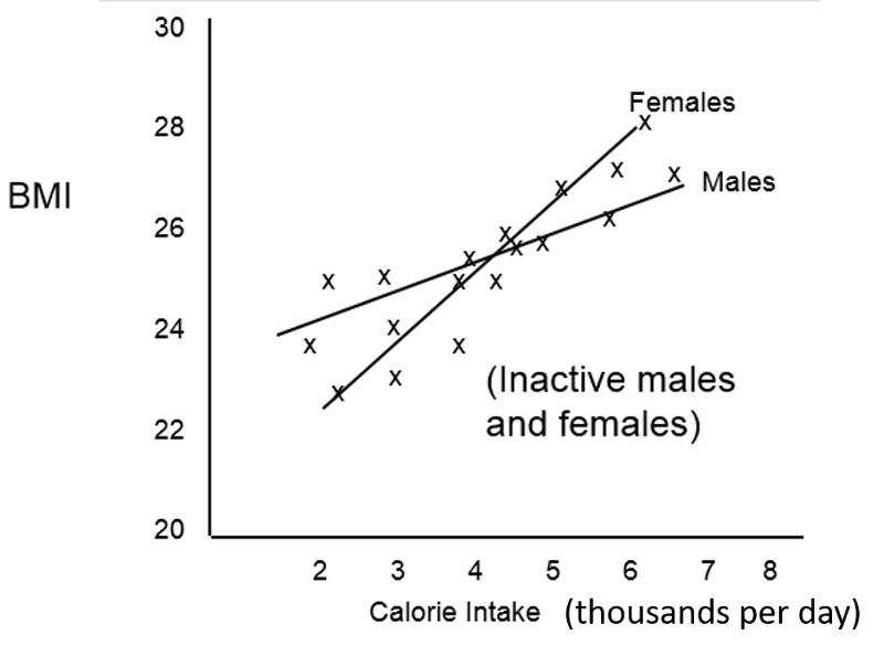
The graph allows us to clearly see what the coefficients are telling us. Suppose we "control for" caloric intake by just focusing on a specific calorie intake, say 5000 calories per day, and also "control" for activity by focusing on activity level 1. If we focus on people with 5000 calorie intakes and activity levels of 1, the effect of being a male compared to a female is an increase of 1.6 units in predicted BMI.
Similarly, if we focus on females with 5000 calorie intakes, the effect of moving from an active female to an inactive female is a predicted increase of 4.2 units in BMI. Finally, at any of the four categories of sex and activity the slope of the line for the effect of caloric intake is 1.5. Thus, the coefficients indicate the incremental change in the dependent variable for each increment in any of the independent variables after controlling for the other variables in the model.
 Test Yourself
Suppose we had observed the following relationship between caloric intake and BMI in inactive males and females. What phenomenon does this depict?