

Distribution of the Sample Mean
The statistic used to estimate the mean of a population, μ, is the sample mean, ![]() .
.
|
If X has a distribution with mean μ, and standard deviation σ, and is approximately normally distributed or n is large, then |

When σ Is Known
If the standard deviation, σ, is known, we can transform ![]() to an approximately standard normal variable, Z:
to an approximately standard normal variable, Z:

Example:
From the previous example, μ=20, and σ=5. Suppose we draw a sample of size n=16 from this population and want to know how likely we are to see a sample average greater than 22, that is P(![]() > 22)?
> 22)?

So the probability that the sample mean will be >22 is the probability that Z is > 1.6 We use the Z table to determine this:
P( > 22) = P(Z > 1.6) = 0.0548.

Exercise: Suppose we were to select a sample of size 49 in the example above instead of n=16. How will this affect the standard error of the mean? How do you think this will affect the probability that the sample mean will be >22? Use the Z table to determine the probability.

When σ Is Unknown
If the standard deviation, σ, is unknown, we cannot transform ![]() to standard normal. However, we can estimate σ using the sample standard deviation, s, and transform
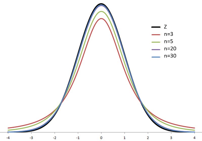
to standard normal. However, we can estimate σ using the sample standard deviation, s, and transform ![]() to a variable with a similar distribution, the t distribution. There are actually many t distributions, indexed by degrees of freedom (df). As the degrees of freedom increase, the t distribution approaches the standard normal distribution.
to a variable with a similar distribution, the t distribution. There are actually many t distributions, indexed by degrees of freedom (df). As the degrees of freedom increase, the t distribution approaches the standard normal distribution.
If X is approximately normally distributed, then

has a t distribution with (n-1) degrees of freedom (df)
Using the t-table
Note: If n is large, then t is approximately normally distributed.
The z table gives detailed correspondences of P(Z>z) for values of z from 0 to 3, by .01 (0.00, 0.01, 0.02, 0.03,…2.99. 3.00). The (one-tailed) probabilities are inside the table, and the critical values of z are in the first column and top row.
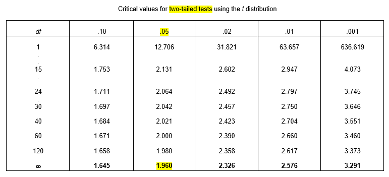
The t-table is presented differently, with separate rows for each df, with columns representing the two-tailed probability, and with the critical value in the inside of the table.
The t-table also provides much less detail; all the information in the z-table is summarized in the last row of the t-table, indexed by df = ∞.
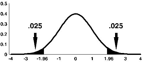
So, if we look at the last row for z=1.96 and follow up to the top row, we find that
P(|Z| > 1.96) = 0.05
Exercise: What is the critical value associated with a two-tailed probability of 0.01?
Now, suppose that we want to know the probability that Z is more extreme than 2.00. The t-table gives us
P(|Z| > 1.96) = 0.05
And
P(|Z| > 2.326) = 0.02
So, all we can say is that P(|Z| > 2.00) is between 2% and 5%, probably closer to 5%! Using the z-table, we found that it was exactly 4.56%.
Example:
In the previous example we drew a sample of n=16 from a population with μ=20 and σ=5. We found that the probability that the sample mean is greater than 22 is P( ![]() > 22) = 0.0548. Suppose that is unknown and we need to use s to estimate it. We find that s = 4. Then we calculate t, which follows a t-distribution with df = (n-1) = 24.
> 22) = 0.0548. Suppose that is unknown and we need to use s to estimate it. We find that s = 4. Then we calculate t, which follows a t-distribution with df = (n-1) = 24.

From the tables we see that the two-tailed probability is between 0.01 and 0.05.
P(|T| > 1.711) = 0.05
And
P(|T| > 2.064) = 0.01
|
To obtain the one-tailed probability, divide the two-tailed probability by 2. |
P(T > 1.711) = ½ P(|T| > 1.711) = ½(0.05) = 0.025
And
P(T > 2.064) = ½ P(|T| > 2.064) = ½(0.01) = 0.005
So the probability that the sample mean is greater than 22 is between 0.005 and 0.025 (or between 0.5% and 2.5%)
Exercise: . If μ=15, s=6, and n=16, what is the probability that ![]() >18 ?
>18 ?