
Type I and Type II Errors
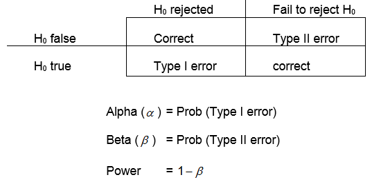
Ideally, both error types (α and β) are small. However, in practice we fix α and choose a sample size n large enough to keep β small (that is, keep power large).
Example:
Two drugs are to be compared in a clinical trial for use in treatment of disease X. Drug A is cheaper than Drug B. Efficacy is measured using a continuous variable, Y, and .H0: μ1=μ2.
Type I error—occurs if the two drugs are truly equally effective, but we conclude that Drug B is better. The consequence is financial loss.
Type II error—occurs if Drug B is truly more effective, but we fail to reject the null hypothesis and conclude there is no significant evidence that the two drugs vary in effectiveness. What is the consequence in this case?
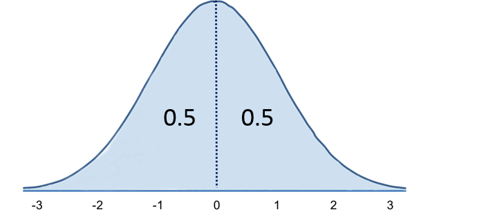
Standard Normal Distribution
Characteristics of the standard normal distribution
The normal distribution is centered at the mean, μ. The degree to which population data values deviate from the mean is given by the standard deviation, σ. 68% of the distribution lies within 1 standard deviation of the mean; 95% lies within two standard deviation of the mean; and 99.9% lies within 3 standard deviations of the mean. The area under the curve is interpreted as probability, with the total area = 1. The normal distribution is symmetric about μ. (i.e., the median and the mean are the same).
The standard normal distribution is a normal distribution with a mean of zero and standard deviation of 1. The standard normal distribution is symmetric around zero: one half of the total area under the curve is on either side of zero. The total area under the curve is equal to one.
For a more detailed discussion of the standard normal distribution see the presentation on this concept in the online module on Probability from BS704.
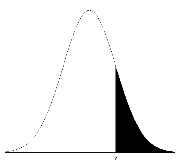
Area in tails of the distribution
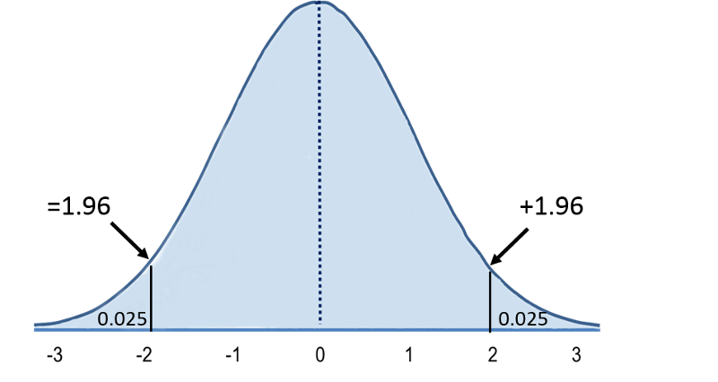
The total area under the curve more than 1.96 units away from zero is equal to 5%. Because the curve is symmetric, there is 2.5% in each tail. Since the total area under the curve = 1, the cumulative probability of Z> +1.96 = 0/025.
A "Z table" provides the area under the normal curve associated with values of z.
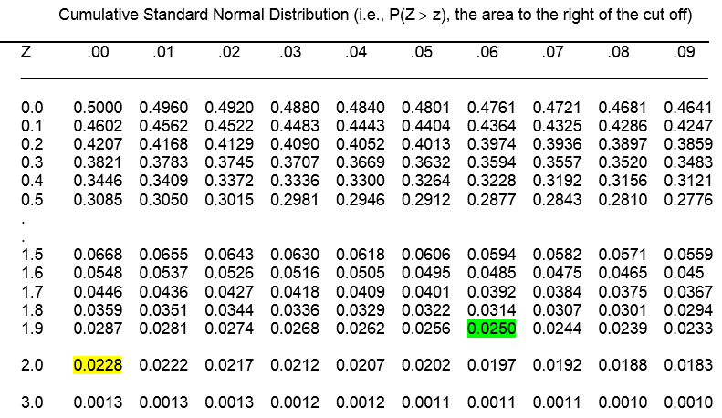
The table below gives cumulative probabilities for various Z scores.
Using the z-table
The z table gives detailed correspondences of P(Z>z) for values of z from 0 to 3, by .01 (0.00, 0.01, 0.02, 0.03,…2.99. 3.00).
So, if we want to know the probability that Z is greater than 2.00, for example, we find the intersection of 2.0 on the left column, and .00 on the top row, and see that P(Z<2.00) = 0.0228.
Alternatively, we can calculate the critical value, z, associated with a given tail probability. So, for example, if we want to find the critical value z, such that P(Z > z) = 0.025, we look inside the table and find it associated with 1.9 on the left column and 0.06 on the top row, so z=1.96. We thus can write,
P(Z > 1.96) = 0.025.
Since the distribution is symmetric, we can simply multiply the one-tailed probabilities to obtain the two-tailed probability:
P(Z < -z OR Z > z) = P(|Z| > z) = 2 * P(Z > z)
Example:
P(|Z| > 1.96) = 2 * P(Z > 1.96 ) = 2 * (0.025) = 0.05, or 5%
Example:
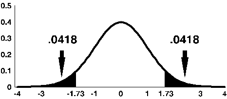
By examining the Z table, we find that about 0.0418 (4.18%) of the area under the curve is above z = 1.73. Thus, for a population that follows the standard normal distribution, approximately 4.18% of the observations will lie above 1.73. The total area under the curve that is more than 1.73 units away from zero is 2(0.0418) or 0.0836 or 8.36%.