SAS - The One Sample t-Test
After successfully completing this module, the student will be able to:
Before observing the data, the null and alternative hypotheses should be stated, a significance level (α) should be chosen (often equal to 0.05), and the test statistic that will summarize the information in the sample should be chosen as well. Based on the hypotheses, test statistic, and sampling distribution of the test statistic, we can find the critical region of the test statistic which is the set of values for the statistical test that show evidence in favor of the alternative hypothesis and against the null hypothesis. This region is chosen such that the probability of the test statistic falling in the critical region when the null hypothesis is correct (Type I error) is equal to the previously chosen level of significance (α).
The test statistic is then calculated:
The p-value, the probability of a test result at least as extreme as the one observed if the null hypothesis was true, can also be calculated.
Example - Paired t-test of change in cholesterol from 1952 to 1962
|
d is the difference in cholesterol for each individual from 1952 to 1962 |
Hypotheses:
H0: There is no change, on average, in cholesterol level from 1952 to 1962
(H0: μd = 0)
H1: There is an average non-zero change in cholesterol level from 1952 to 1962
(H1: μd ≠ 0)
Test statistic:
![]()
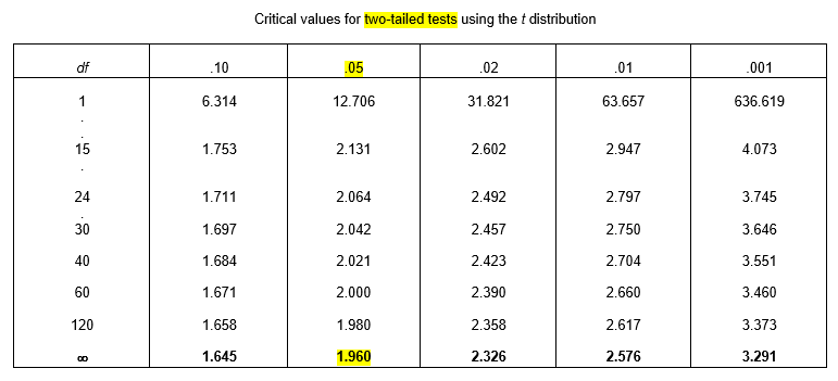
Decision rule: Reject H0 at α=0.05 if |t| > 2.093
The decision rule is constructed from the sampling distribution for the test statistic t. For this example, the sampling distribution of the test statistic, t, is a student t-distribution with 19 degrees of freedom. The critical value 2.093 can be read from a table for the t-distribution.
Results:
![]() .
.
Conclusion:
Cholesterol levels decreased, on average, 69.8 units from 1952 to 1962. For a significance level of 0.05 and 19 degrees of freedom, the critical value for the t-test is 2.093. Since the absolute value of our test statistic (6.70) is greater than the critical value (2.093) we reject the null hypothesis and conclude that there is on average a non-zero change in cholesterol from 1952 to 1962.
Note that this summary includes:
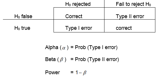
Ideally, both error types (α and β) are small. However, in practice we fix α and choose a sample size n large enough to keep β small (that is, keep power large).
Example:
Two drugs are to be compared in a clinical trial for use in treatment of disease X. Drug A is cheaper than Drug B. Efficacy is measured using a continuous variable, Y, and .H0: μ1=μ2.
Type I error—occurs if the two drugs are truly equally effective, but we conclude that Drug B is better. The consequence is financial loss.
Type II error—occurs if Drug B is truly more effective, but we fail to reject the null hypothesis and conclude there is no significant evidence that the two drugs vary in effectiveness. What is the consequence in this case?
The normal distribution is centered at the mean, μ. The degree to which population data values deviate from the mean is given by the standard deviation, σ. 68% of the distribution lies within 1 standard deviation of the mean; 95% lies within two standard deviation of the mean; and 99.9% lies within 3 standard deviations of the mean. The area under the curve is interpreted as probability, with the total area = 1. The normal distribution is symmetric about μ. (i.e., the median and the mean are the same).
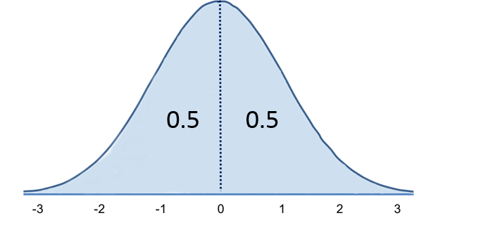
The standard normal distribution is a normal distribution with a mean of zero and standard deviation of 1. The standard normal distribution is symmetric around zero: one half of the total area under the curve is on either side of zero. The total area under the curve is equal to one.
For a more detailed discussion of the standard normal distribution see the presentation on this concept in the online module on Probability from BS704.
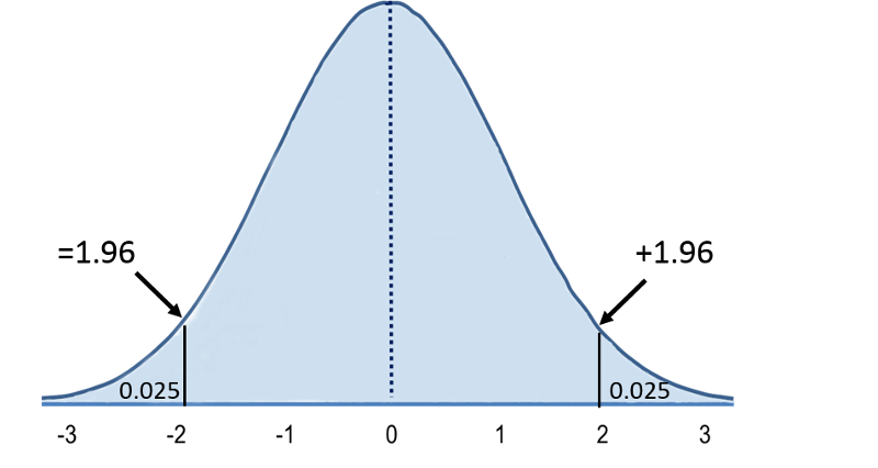
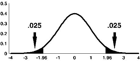
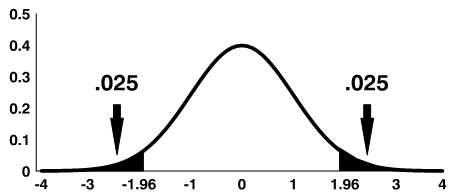
The total area under the curve more than 1.96 units away from zero is equal to 5%. Because the curve is symmetric, there is 2.5% in each tail. Since the total area under the curve = 1, the cumulative probability of Z> +1.96 = 0/025.
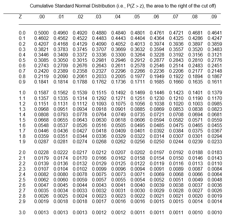
A "Z table" provides the area under the normal curve associated with values of z.
The table below gives cumulative probabilities for various Z scores.
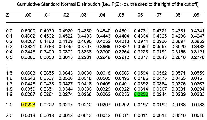
Using the z-table
The z table gives detailed correspondences of P(Z>z) for values of z from 0 to 3, by .01 (0.00, 0.01, 0.02, 0.03,…2.99. 3.00).
So, if we want to know the probability that Z is greater than 2.00, for example, we find the intersection of 2.0 on the left column, and .00 on the top row, and see that P(Z<2.00) = 0.0228.
Alternatively, we can calculate the critical value, z, associated with a given tail probability. So, for example, if we want to find the critical value z, such that P(Z > z) = 0.025, we look inside the table and find it associated with 1.9 on the left column and 0.06 on the top row, so z=1.96. We thus can write,
P(Z > 1.96) = 0.025.
Since the distribution is symmetric, we can simply multiply the one-tailed probabilities to obtain the two-tailed probability:
P(Z < -z OR Z > z) = P(|Z| > z) = 2 * P(Z > z)
Example:
P(|Z| > 1.96) = 2 * P(Z > 1.96 ) = 2 * (0.025) = 0.05, or 5%
Example:
By examining the Z table, we find that about 0.0418 (4.18%) of the area under the curve is above z = 1.73. Thus, for a population that follows the standard normal distribution, approximately 4.18% of the observations will lie above 1.73. The total area under the curve that is more than 1.73 units away from zero is 2(0.0418) or 0.0836 or 8.36%.

Given a normally distributed variable X with a population mean of and a population standard deviation of σ
![]()
Example:
Suppose a normally distributed population has μ=20, σ=5, and we want to know what percentage of the distribution is above X = 30.

This is equivalent to asking how much of the distribution is more than 2 standard deviations above the mean, or what is the probability that X is more than 2 standard deviations above the mean.
From the Z table, we can see that 2.28% of the distribution lies above Z = 2.00. Thus, 2.28% of the population which has a normal distribution with a μ of 20 and a σ of 5 lies above X = 30.
We can write this as
P(X > 30) = P(Z > 2) = 0.0228, or 2.28%
The statistic used to estimate the mean of a population, μ, is the sample mean, ![]() .
.
|
If X has a distribution with mean μ, and standard deviation σ, and is approximately normally distributed or n is large, then |
When σ Is Known
If the standard deviation, σ, is known, we can transform ![]() to an approximately standard normal variable, Z:
to an approximately standard normal variable, Z:

Example:
From the previous example, μ=20, and σ=5. Suppose we draw a sample of size n=16 from this population and want to know how likely we are to see a sample average greater than 22, that is P(![]() > 22)?
> 22)?

So the probability that the sample mean will be >22 is the probability that Z is > 1.6 We use the Z table to determine this:
P( > 22) = P(Z > 1.6) = 0.0548.

Exercise: Suppose we were to select a sample of size 49 in the example above instead of n=16. How will this affect the standard error of the mean? How do you think this will affect the probability that the sample mean will be >22? Use the Z table to determine the probability.
Answer
When σ Is Unknown
If the standard deviation, σ, is unknown, we cannot transform ![]() to standard normal. However, we can estimate σ using the sample standard deviation, s, and transform
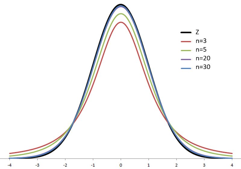
to standard normal. However, we can estimate σ using the sample standard deviation, s, and transform ![]() to a variable with a similar distribution, the t distribution. There are actually many t distributions, indexed by degrees of freedom (df). As the degrees of freedom increase, the t distribution approaches the standard normal distribution.
to a variable with a similar distribution, the t distribution. There are actually many t distributions, indexed by degrees of freedom (df). As the degrees of freedom increase, the t distribution approaches the standard normal distribution.
If X is approximately normally distributed, then

has a t distribution with (n-1) degrees of freedom (df)
Note: If n is large, then t is approximately normally distributed.
The z table gives detailed correspondences of P(Z>z) for values of z from 0 to 3, by .01 (0.00, 0.01, 0.02, 0.03,…2.99. 3.00). The (one-tailed) probabilities are inside the table, and the critical values of z are in the first column and top row.
The t-table is presented differently, with separate rows for each df, with columns representing the two-tailed probability, and with the critical value in the inside of the table.
The t-table also provides much less detail; all the information in the z-table is summarized in the last row of the t-table, indexed by df = ∞.
So, if we look at the last row for z=1.96 and follow up to the top row, we find that
P(|Z| > 1.96) = 0.05
Exercise: What is the critical value associated with a two-tailed probability of 0.01?
Answer
Now, suppose that we want to know the probability that Z is more extreme than 2.00. The t-table gives us
P(|Z| > 1.96) = 0.05
And
P(|Z| > 2.326) = 0.02
So, all we can say is that P(|Z| > 2.00) is between 2% and 5%, probably closer to 5%! Using the z-table, we found that it was exactly 4.56%.
Example:
In the previous example we drew a sample of n=16 from a population with μ=20 and σ=5. We found that the probability that the sample mean is greater than 22 is P( ![]() > 22) = 0.0548. Suppose that is unknown and we need to use s to estimate it. We find that s = 4. Then we calculate t, which follows a t-distribution with df = (n-1) = 24.
> 22) = 0.0548. Suppose that is unknown and we need to use s to estimate it. We find that s = 4. Then we calculate t, which follows a t-distribution with df = (n-1) = 24.

From the tables we see that the two-tailed probability is between 0.01 and 0.05.
P(|T| > 1.711) = 0.05
And
P(|T| > 2.064) = 0.01
|
To obtain the one-tailed probability, divide the two-tailed probability by 2. |
P(T > 1.711) = ½ P(|T| > 1.711) = ½(0.05) = 0.025
And
P(T > 2.064) = ½ P(|T| > 2.064) = ½(0.01) = 0.005
So the probability that the sample mean is greater than 22 is between 0.005 and 0.025 (or between 0.5% and 2.5%)
Exercise: . If μ=15, s=6, and n=16, what is the probability that ![]() >18 ?
>18 ?
Answer
A one sample test of means compares the mean of a sample to a pre-specified value and tests for a deviation from that value. For example we might know that the average birth weight for white babies in the US is 3,410 grams and wish to compare the average birth weight of a sample of black babies to this value.
Assumptions
Hypothesis:

where μ0 is a pre-specified value (in our case this would be 3,410 grams).
Test Statistic

Using the significance level of 0.05, we reject the null hypothesis if z is greater than 1.96 or less than -1.96.

Using the significance level of 0.05, we reject the null hypothesis if |t| is greater than the critical value from a t-distribution with df = n-1.
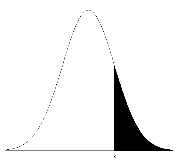
Note: The shaded area is referred to as the critical region or rejection region.
We can also calculate a 95% confidence interval around the mean. The general form for a confidence interval around the mean, if σ is unknown, is
![]()
For a two-sided 95% confidence interval, use the table of the t-distribution (found at the end of the section) to select the appropriate critical value of t for the two-sided α=0.05.
Example: one sample t-test
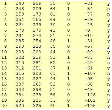
Recall the data used in module 3 in the data file "dixonmassey."
data dixonmassey;
input Obs chol52 chol62 age cor dchol agelt50 $;
datalines;
;
Many doctors recommend having a total cholesterol level below 200 mg/dl. We will test to see if the 1952 population from which the Dixon and Massey sample was gathered is statistically different, on average, from this recommended level.
Calculate:

|t| > 2.093 so we reject H0
The 95% confidence limits around the mean are
311.15 ± (2.093)(64.3929/√20)
311.15 ± 30.14
(281.01, 341.29)
proc ttest data=name h0=μ0 alpha=α;
var var;
run;
SAS uses the stated α for the level of confidence (for example, α=0.05 will result in 95% confidence limits). For the hypothesis test, however, it does not compute critical values associated with the given α, and compare the t-statistic to the critical value. Rather, SAS will provide the p-value, the probability that T is more extreme than observed t. The decision rule, "reject if |t| > critical value associated with α" is equivalent to "reject if p < α."
|
SAS will provide the p-value, the probability that T is more extreme than observed t. The decision rule, "reject if |t| > critical value associated with α" is equivalent to "reject if p < α." |
Example:
proc ttest data=dixonmassey h0=200 alpha=0.05;
var chol52;
title 'One Sample t-test with proc ttest';
title2 'Testing if the sample of cholesterol levels in 1952 is statistically different from 200' ;
run;
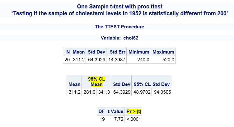
As in our hand calculations, t = 7.72, and we reject H0 (because p<0.0001 which is < 0.05, our selected α level).
The mean cholesterol in 1952 was 311.2, with 95% confidence limits (281.0, 341.3).
A paired t-test is used when we are interested in the difference between two variables for the same subject.
Often the two variables are separated by time. For example, in the Dixon and Massey data set we have cholesterol levels in 1952 and cholesterol levels in 1962 for each subject. We may be interested in the difference in cholesterol levels between these two time points.
However, sometimes the two variables are separated by something other than time. For example, subjects with h ACL tears may be asked to balance on their leg with the torn ACL and then to balance again on their leg without the torn ACL. Then, for each subject, we can then calculate the difference in balancing time between the two legs.
|
Since we are ultimately concerned with the difference between two measures in one sample, the paired t-test reduces to the one sample t-test. |
Null Hypothesis: H0: μd = 0
Alternative Hypothesis: H1: μd ≠ 0
Point Estimate:![]() (the sample mean difference) is the point estimate of .μd
(the sample mean difference) is the point estimate of .μd
Test statistic:

Note that the standard error of ![]() is
is ![]() where sd is the standard deviation of the differences.
where sd is the standard deviation of the differences.
As before, we compare the t-statistic to the critical value of t (which can be found in the table using degrees of freedom and the pre-selected level of significance, α). If the absolute value of the calculated t-statistic is larger than the critical value of t, we reject the null hypothesis.
Confidence Intervals
We can also calculate a 95% confidence interval around the difference in means. The general form for a confidence interval around a difference in means is
![]()
For a two-sided 95% confidence interval, use the table of the t-distribution (found at the end of the section) to select the appropriate critical value of t for the two-sided α=0.05. .
Example:
Suppose we wish to determine if the cholesterol levels of the men in Dixon and Massey study changed from 1952 to 1962. We will use the paired t-test.

For α = 0.05 and 19 df, the critical value of t is 2.093. Since | -6.7| > 2.093, we reject H0 and state that we have significant evidence that the average difference in cholesterol from 1952 to 1962 is NOT 0. Specifically, there was an average decrease of 69.8 from 1952 to 1962.
To perform a paired t-test in SAS, comparing variables X1 and X2 measured on the same people, you can first create the difference as we did above, and perform a one sample t-test of:
![]()
data pairedtest; set original;
d=x1-x2;
run;
proc ttest data=pairedtest h0=0;
var d;
run;
Hypotheses:
First, create the difference, dchol.
data dm; set dixonmassey;
dchol=chol62-chol52;
run;
proc ttest data=dm;
title 'Paired t-test with proc ttest, using dchol variable';
var dchol;
run;
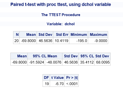
Again, we reject H0 (because p<0.05) and state that we have significant evidence that cholesterol levels changed from 1952 to 1962, with an average decrease of 69.8 units, with 95% confidence limits of (-91.6, -48.0).
Alternatively, we can (only for a test of H0: μd = 0) use proc means:
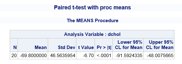
proc means data=pairedtest n mean std t prt clm;
title 'Paired t-test with proc means';
var dchol;
run;
Note that the t option produces the t statistic for testing the null hypothesis that the mean of a variable is equal to zero, and the prt option gives the associated p-value. The clm option produces a 95% confidence interval for the mean. In this case, where the variable is a difference, dchol, the null hypothesis is that the mean difference is zero and the 95% confidence interval is for the mean difference.
proc means data=dm n mean std t prt clm;
title 'Paired t-test with proc means';
var dchol;
run;
A third method is to use the original data with the paired option in proc t-test:
proc ttest data=original;
title 'Paired t-test with proc ttest, paired statement';
paired x1*x2;
run;
This produces identical output to the t-test on dchol.
Example:
proc ttest data=work.dm;
title 'Paired t-test with proc ttest, paired statement';
paired chol62*chol52;
run;
We conducted a paired t-test to determine whether, on average, there was a change in cholesterol from 1952 to 1962.
Note that this report includes: