


Issues in Estimating Sample Size for Hypothesis Testing
In the module on hypothesis testing for means and proportions, we introduced techniques for means, proportions, differences in means, and differences in proportions. While each test involved details that were specific to the outcome of interest (e.g., continuous or dichotomous) and to the number of comparison groups (one, two, more than two), there were common elements to each test. For example, in each test of hypothesis, there are two errors that can be committed. The first is called a Type I error and refers to the situation where we incorrectly reject H0 when in fact it is true. In the first step of any test of hypothesis, we select a level of significance, α , and α = P(Type I error) = P(Reject H0 | H0 is true). Because we purposely select a small value for α , we control the probability of committing a Type I error. The second type of error is called a Type II error and it is defined as the probability we do not reject H0 when it is false. The probability of a Type II error is denoted β , and β =P(Type II error) = P(Do not Reject H0 | H0 is false). In hypothesis testing, we usually focus on power, which is defined as the probability that we reject H0 when it is false, i.e., power = 1- β = P(Reject H0 | H0 is false). Power is the probability that a test correctly rejects a false null hypothesis. A good test is one with low probability of committing a Type I error (i.e., small α ) and high power (i.e., small β, high power).
Here we present formulas to determine the sample size required to ensure that a test has high power. The sample size computations depend on the level of significance, aα, the desired power of the test (equivalent to 1-β), the variability of the outcome, and the effect size. The effect size is the difference in the parameter of interest that represents a clinically meaningful difference. Similar to the margin of error in confidence interval applications, the effect size is determined based on clinical or practical criteria and not statistical criteria.
The concept of statistical power can be difficult to grasp. Before presenting the formulas to determine the sample sizes required to ensure high power in a test, we will first discuss power from a conceptual point of view.
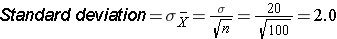
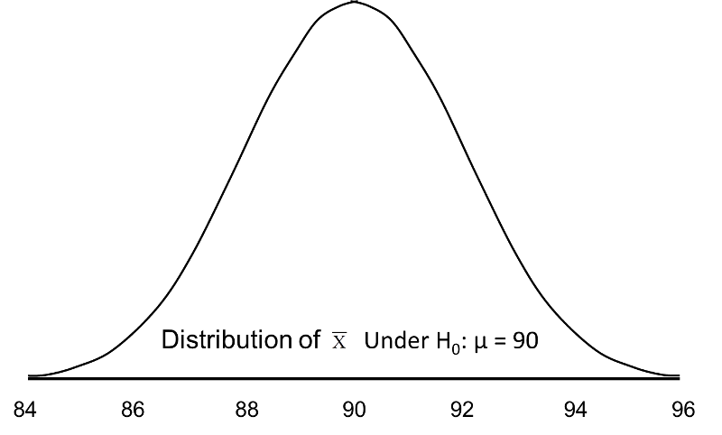
Suppose we want to test the following hypotheses at aα=0.05: H0: μ = 90 versus H1: μ ≠ 90. To test the hypotheses, suppose we select a sample of size n=100. For this example, assume that the standard deviation of the outcome is σ=20. We compute the sample mean and then must decide whether the sample mean provides evidence to support the alternative hypothesis or not. This is done by computing a test statistic and comparing the test statistic to an appropriate critical value. If the null hypothesis is true (μ=90), then we are likely to select a sample whose mean is close in value to 90. However, it is also possible to select a sample whose mean is much larger or much smaller than 90. Recall from the Central Limit Theorem (see page 11 in the module on Probability), that for large n (here n=100 is sufficiently large), the distribution of the sample means is approximately normal with a mean of


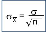
and
If the null hypothesis is true, it is possible to observe any sample mean shown in the figure below; all are possible under H0: μ = 90.
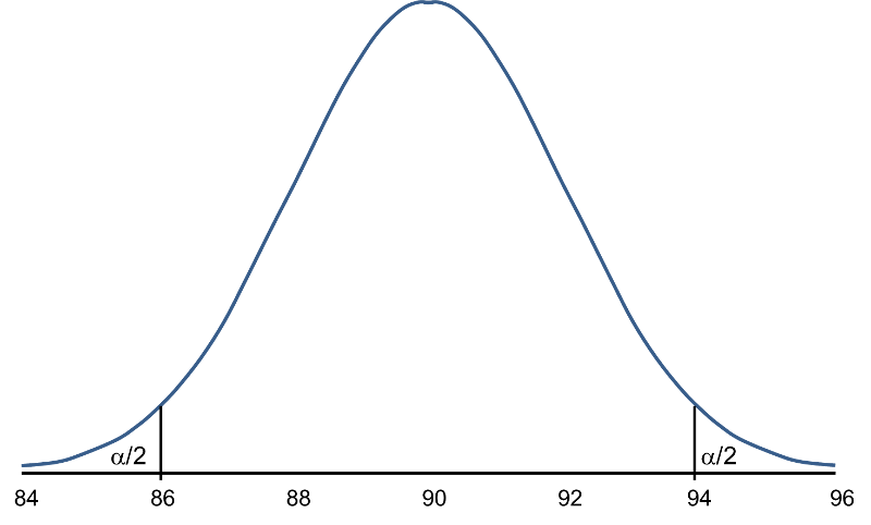
When we set up the decision rule for our test of hypothesis, we determine critical values based on α=0.05 and a two-sided test. When we run tests of hypotheses, we usually standardize the data (e.g., convert to Z or t) and the critical values are appropriate values from the probability distribution used in the test. To facilitate interpretation, we will continue this discussion with ![]() as opposed to Z. The critical values for a two-sided test with α=0.05 are 86.06 and 93.92 (these values correspond to -1.96 and 1.96, respectively, on the Z scale), so the decision rule is as follows: Reject H0 if
as opposed to Z. The critical values for a two-sided test with α=0.05 are 86.06 and 93.92 (these values correspond to -1.96 and 1.96, respectively, on the Z scale), so the decision rule is as follows: Reject H0 if ![]() < 86.06 or if
< 86.06 or if ![]() > 93.92. The rejection region is shown in the tails of the figure below.
> 93.92. The rejection region is shown in the tails of the figure below.
Rejection Region for Test H0: μ = 90 versus H1: μ ≠ 90 at α =0.05
 .
.
The areas in the two tails of the curve represent the probability of a Type I Error, α= 0.05. This concept was discussed in the module on Hypothesis Testing.
Now, suppose that the alternative hypothesis, H1, is true (i.e., μ ≠ 90) and that the true mean is actually 94. The figure below shows the distributions of the sample mean under the null and alternative hypotheses.The values of the sample mean are shown along the horizontal axis.
Distribution of Under H0: μ = 90 and Under H1: μ = 94
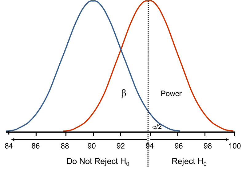
If the true mean is 94, then the alternative hypothesis is true. In our test, we selected α = 0.05 and reject H0 if the observed sample mean exceeds 93.92 (focusing on the upper tail of the rejection region for now). The critical value (93.92) is indicated by the vertical line. The probability of a Type II error is denoted β, and β = P(Do not Reject H0 | H0 is false), i.e., the probability of not rejecting the null hypothesis if the null hypothesis were true. β is shown in the figure above as the area under the rightmost curve (H1) to the left of the vertical line (where we do not reject H0). Power is defined as 1- β = P(Reject H0 | H0 is false) and is shown in the figure as the area under the rightmost curve (H1) to the right of the vertical line (where we reject H0 ).
Note that β and power are related to α, the variability of the outcome and the effect size. From the figure above we can see what happens to β and power if we increase α. Suppose, for example, we increase α to α=0.10.The upper critical value would be 92.56 instead of 93.92. The vertical line would shift to the left, increasing α, decreasing β and increasing power. While a better test is one with higher power, it is not advisable to increase α as a means to increase power. Nonetheless, there is a direct relationship between α and power (as α increases, so does power).
β and power are also related to the variability of the outcome and to the effect size. The effect size is the difference in the parameter of interest (e.g., μ) that represents a clinically meaningful difference. The figure above graphically displays α, β, and power when the difference in the mean under the null as compared to the alternative hypothesis is 4 units (i.e., 90 versus 94). The figure below shows the same components for the situation where the mean under the alternative hypothesis is 98.
Figure - Distribution of Under H0: μ = 90 and Under H1: μ = 98.
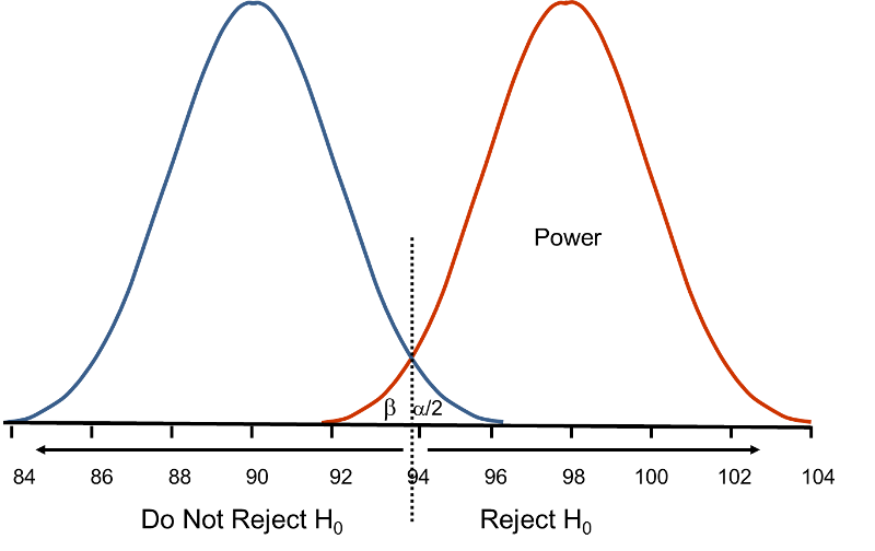
Notice that there is much higher power when there is a larger difference between the mean under H0 as compared to H1 (i.e., 90 versus 98). A statistical test is much more likely to reject the null hypothesis in favor of the alternative if the true mean is 98 than if the true mean is 94. Notice also in this case that there is little overlap in the distributions under the null and alternative hypotheses. If a sample mean of 97 or higher is observed it is very unlikely that it came from a distribution whose mean is 90. In the previous figure for H0: μ = 90 and H1: μ = 94, if we observed a sample mean of 93, for example, it would not be as clear as to whether it came from a distribution whose mean is 90 or one whose mean is 94.
Ensuring That a Test Has High Power
In designing studies most people consider power of 80% or 90% (just as we generally use 95% as the confidence level for confidence interval estimates). The inputs for the sample size formulas include the desired power, the level of significance and the effect size. The effect size is selected to represent a clinically meaningful or practically important difference in the parameter of interest, as we will illustrate.
The formulas we present below produce the minimum sample size to ensure that the test of hypothesis will have a specified probability of rejecting the null hypothesis when it is false (i.e., a specified power). In planning studies, investigators again must account for attrition or loss to follow-up. The formulas shown below produce the number of participants needed with complete data, and we will illustrate how attrition is addressed in planning studies.