Data Analysis
Data analysis is the means through which investigators can communicate valuable information about the exposure-disease pathway. In other words, what is there an association between the exposure of interest and the health outcome of interest? If so, what is the nature of this relationship? While statistical numbers and visual displays are an important component of the data analysis, there are other aspects. When thinking about data analysis, the items below provide a more comprehensive look at data analysis.
- Develop a plan for managing and analyzing data
- Evaluate quality of data and determine final sample values
- Look at the data! Graphical displays such as histograms (distribution) and scatter plots
- Descriptive statistics (n, mean, median, standard deviation, range)
- Consider possible exposure indices of interest (intensity, duration, cumulative, etc.)
Maintaining the integrity of data collected and having a protocol for how that data will be coded and analyzed is essential to any exposure assessment. A data management plan is a formal document developed by investigators in the design phase of a study that describes how investigators will handle the data during and after the study. There are three key stages that can be considered integral to any data management plan: preparatory, data organization, and analysis and dissemination .
Quality Assurance/Quality Control
Think about the multiple steps involved in measuring an exposure of interest. With the use of measuring equipment, a process is employed to set up in the "field" often followed by some sort of transport from the field to a lab or some other location in order to extract and analyze information about the exposure. There are many opportunities for contamination to occur that can affect the results of the exposure data. In order to minimize errors that may be introduced in the exposure collection process, there are several methods that can be incorporated into the study protocol.
According to the EPA, the "primary purpose of blanks is to trace sources of artificially introduced contamination." In addition to blanks, investigators can utilize different sampling methods to assess and correct for measurement error introduced during the data collection and sampling analysis process. Review the activity below for definitions and examples of these quality assurance/quality control measures.
Measures for Quality Assurance/Quality Control
- Field Blanks: A clean sample, such as distilled water, carried to the sampling site, exposed to sampling conditions (e.g. bottle caps removed, preservatives added) and returned to the laboratory and treated as an environmental sample. Field blanks are used to check for analytical artifacts and/or background introduced by sampling and analytical procedures.
- Lab Blanks: A sample consisting of reagent(s) without the target analyte or sample matrix that is introduced into the analytical procedure at the appropriate point and carried through all subsequent steps. The goal is to determine the contribution of the reagent(s) and all of the involved analytical steps to error in the observed value.
- Equipment Blanks: A clean sample that is collected in a sample container with the sample-collection device and returned to the laboratory as a sample. Sampling equipment blanks are used to check the cleanliness of sampling devices.
- Trip Blanks: A clean sample of matrix that is carried to the sampling site and transported to the laboratory for analysis without having been exposed to the sampling procedures.
- Duplicate Samples: Two samples taken from and representative of the sample population and carried through all the steps of the sampling and analytical procedures in an indentical manner. Duplicate samples are used to assess variance of the total method including sampling and analysis.
- Matrix Spike Samples: A sample prepared by adding a known mass of target analyte to a specified amount of matrix sample for which an independent estimate of target analyte concentration is available. Spiked samples are used, for example, to determine the effect of the matrix on a method's recovery efficiency.
- Split Samples: Two or more representative portions taken from a sample or subsample and analyzed by different analysts or laboratories. Split samples are used to replicate the measurement of the variable(s) of interest.
- Internal Standards: A standard added to a test portion of a sample in a known amount and carried through the entire determination procedure as a reference for calibration and controlling the precision and biased of the applied analytical method.
- Reference Materials: A material or substance, one or more properties of which are sufficiently well established to be used for the calibration of an apparatus, the assessment of a measurement method, or assigning values to materials.
- QA/QC Samples: An uncontaminated sample matrix spiked with known amounts of analytes from a source independent from the calibration standards. It is generally used to establish intralaboratory or analyst specific precision and bias or to assess the performance of all or a portion of the measurement system.
Sample Value Determination
The processes involved in collecting, preparing, and analyzing sample concentrations can yield measurements that are different from the true sample value as a result of contamination or errors with the sampling method. Sample values must be evaluated and possibly corrected for contamination, accuracy, and precision. Corrected sample concentrations represent the "true" sample level without any effects from sample preparation, analysis, or collection
Analytical instruments and techniques can produce a signal even when analyzing a blank, which is why a limit of detection must be established. The limit of detection, or detection limit, is the smallest amount of a substance that can be determined to be significantly different from background noise or a blank sample. There are several different detection limits that are commonly used. The list below highlights detection limits based on the instrument used to analyze the substance or the overall method.
- Instrumental LOD: It is the smallest concentration of a sample or sample extract that can be determined on the instrument. The instrument LOD is typically determined using lab blanks and is often calculated as three times the standard deviation of the blanks.
- Method LOD: In trace analysis, there is often additional steps involved beyond analyzing an clean sample (e.g. remove unwanted matrix components, extract and concentrate the analyte, etc.). The method LOD is the smallest sample concentration that can be measured by the overall method. It includes variability from the instrument. It is typically determined using field blanks and calculated as three times the standard deviation of the blanks.
Common approaches for analyzing results below the detection limit:
- Use reported value
- Substitute with MDL/2 (data with normal distribution)
- Substitute with MDL/√2 (data with lognormal distribution)
Accuracy & Precision
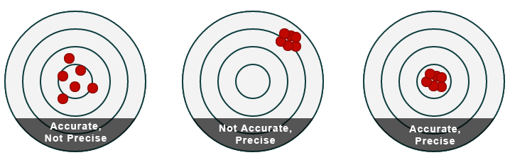
By assessing accuracy, we address the question: what is the "true value" relative to the sample value? The goal is to account for any measurement error that may affect the sample value by causing it to deviate from the true value. When assessing precision, the question becomes: how much variability exists among the sample values? The image below illustrates different scenarios of accuracy and precision with the bulls eye representing the "true value" or "true exposure."
There are several methods that can be employed in order to assess the level of accuracy and precision in a study. Examples are provided in the diagram below.
Assessing Accuracy
- Method 1: Percent Error
- The formula below calculates the percent error, which allows investigators to determine the degree of agreement between the sample value and a reference or true value. (E = Experimental value, A = Actual/True value)
- The formula below calculates the percent error, which allows investigators to determine the degree of agreement between the sample value and a reference or true value. (E = Experimental value, A = Actual/True value)
- Method 2: Regression
- The experimental method employed to measure an exposure can be calibrated with a reference method. Then the relationship between the experimental and reference methods can be assessed using linear regression.
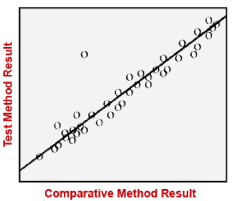
- The experimental method employed to measure an exposure can be calibrated with a reference method. Then the relationship between the experimental and reference methods can be assessed using linear regression.
Assessing Precision
- Method 1: Percent Precision
- The formula below calculates the percent precision, where RMSE (root mean standard error) measures the difference between a regular sample and a collocated sample.
- The formula below calculates the percent precision, where RMSE (root mean standard error) measures the difference between a regular sample and a collocated sample.
- Method 2: Percent Difference
- The percent difference shown below indicates the difference between two collocated samples and is expressed as a percentage of the mean.
- The percent difference shown below indicates the difference between two collocated samples and is expressed as a percentage of the mean.
- Method 3: Coefficient of Variation
- It shows the extent of variability in relation to the mean of the population.
- It shows the extent of variability in relation to the mean of the population.
Confounding & Effect Modification
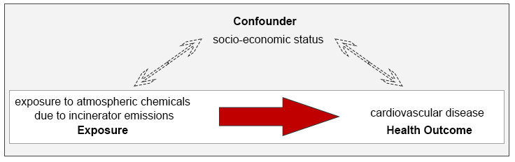
For studies assessing the relationship between exposure and an outcome, confounding and effect modification are two factors that can affect the results of the study by over- or underestimating the true magnitude of the effect. Confounding occurs when variables other than the exposure might explain the relationship seen between incinerators and poor health outcomes. The illustration below highlights a scenario in which investigators wish to assess the relationship between incinerator emissions and cardiovascular disease. In this case, socio-economic status (SES) can be a confounding factor since it is associated with both the exposure and the health outcome independently.
Effect measure modification is when the magnitude of effect seen between an exposure and health outcome is somehow modified by a third variable. Some medications are known to be more effective in men compared to women, making sex an effect modifier in such cases. A study looking at the effects of fluoride exposure and hip fractures should consider the fact that elderly women are at increased risk of hip fractures when compared to men. To learn more about how to address confounding and effect modification in a study, you may review the module on confounding & effect modification.
The table below highlights some measures for minimizing and controlling for confounding. Note that effect modifiers can only be reported and cannot be adjusted via analytical techniques.
Minimizing and Controlling for Confounding
- Study Design
- When recruiting or identifying study participants, investigators can restrict admission into the study based on the confounder. (e.g. women between the ages of 25-40 if the confounders are age and sex).
- Matching is another method in which investigators can match subjects in the exposure groups based on the confounder (e.g. for every exposed women between the ages of 25-40, investigators enroll an unexposed women between the ages of 25-40).
- Randomization is a method that can be used for clinical trials in which study participants are randomly allocated to the exposed or the unexposed group, which tends to evenly distribute both known and unknown confounding variables between groups.
- Analysis Phase
- Investigators can stratify the data based on the confounding variable(s) and measure the magnitude of the association separately (e.g. calculate risk estimates in women 25-40 and women 40+ separately). If confounding is present, a pooled risk estimate can be calculated using the Cochran-Mantel-Haenszel method.
- Multiple regression analysis is also used to assess whether confounding exists. Since multiple linear regression analysis allows us to estimate the association between a given independent variable and the outcome holding all other variables constant, it provides a way of adjusting for (or accounting for) potentially confounding variables that have been included in the model.
*Analytical techniques can be utilized to adjust for confounding given investigators have collected information on the confounder such as by collecting baseline characteristics.
Presenting the Data
When it comes to the findings of an exposure assessment, numbers alone often do not tell the whole story since valuable information such as trends (e.g. dose-response relationships) often require some visual representation. Investigators must identify the most meaningful way to communicate the story being told by the data. One of the key considerations when presenting data is to ensure that specific objectives and aims have been identified (the design portion of the study) and that any analyses performed addresses those objectives.
The following are some common ways data may be evaluated and subsequently presented in exposure assessments. For more information, you may view a module on data presentation.
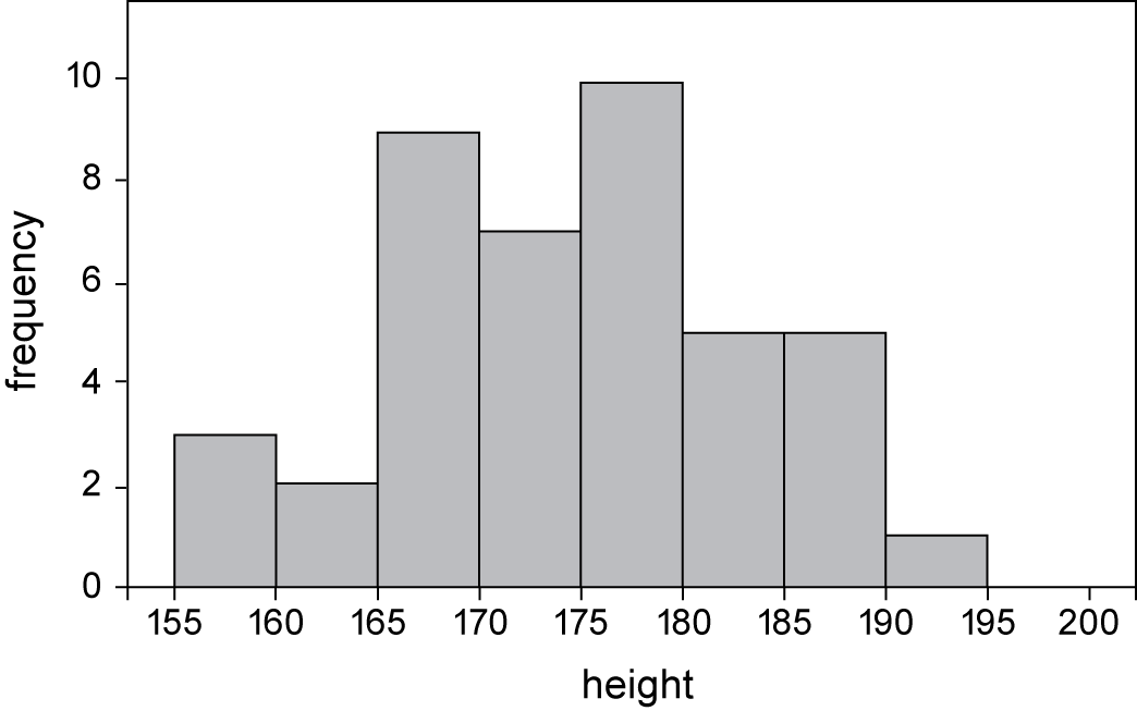
Distribution
Frequency distribution tables can be used to display the frequency of various outcomes in a sample. The goal in presenting the distribution of the data is to show the number of observations of a variable for a given interval. A common visual representation of the distribution is a histogram shown below.
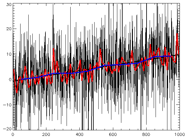
Time Series
A time series consists of a sequence of data points that generally consists of continuous data over a given time interval. When data is collected for a given variable over a period of time, such data can be presented by a line chart as shown below. Line charts that accompany times series data often depict a best-fit trend.
Summary Statistics
This consists of descriptive statistics that are used to summarize a set of observations. It is often used to communciated the largest amount of information as simply as possible and includes the following: location, spread, and dependence. This includes things like the arithmetic mean, median, standard deviation, range, shape of distribution, and a measure of statistical dependence (e.g. correlation coefficient) if more than one variable is present.
Summary Statistics Source: Zwack, Leonard M et al. Modeling Spatial Patterns of Traffic-Related Air Pollutants in Complex Urban Terrain
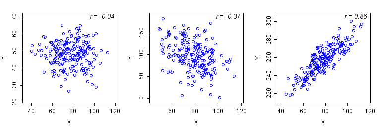
Correlation Data
Scatterplots are a common graphical display used to illustrate the relationship (correlation) between two variables. A correlation coefficient is often calculated to measure the strength and direction of the linear relationship between two variables. Shown below are two scatterplots in which the correlation is stronger on the right and positive, whereas the graph on the left shows a weaker correlation that happens to be negative.
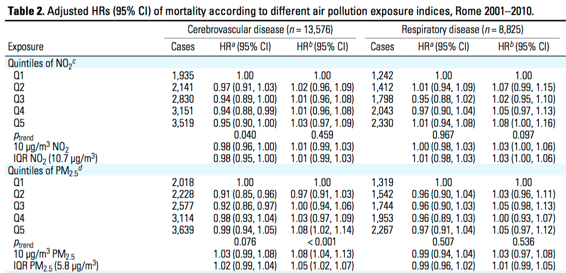
Exposure Indices
Exposure indices can be helpful in establishing a dose-response relationship since many levels or a range of exposure can be assessed. Exposure indices can be classified such as by job category or they can be presented by quantitative values that take into consideration more than one factor. Shown below is an example in which exposure indices are established based on which quintile of exposure to air pollutants NO2 and PM2.5 a given case belongs.
Image Source: Cesaroni, Giulia et al. Long-Term Exposure to Urban Air Pollution and Mortality in a Cohort of More than a Million Adults in Rome.
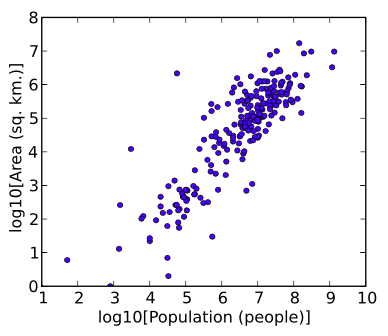
Log Transformation
Data transformations in which data points are replaced with their log value. Such transformations are useful when values range over several orders of magnitude, and when the data is widely distributed or skewed. Another reason for log transforming is to establish a more linear relationship for the purposes of logistic or linear regression analyses.
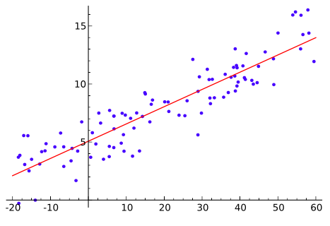
Regression Analysis
Regression analysis is a statistical process for measuring relationships among variables. Regression analysis generally helps to assess the relationship between a dependent variable and one or more independent variables.