Estimating the Survival Function

---

There are several different ways to estimate a survival function or a survival curve. There are a number of popular parametric methods that are used to model survival data, and they differ in terms of the assumptions that are made about the distribution of survival times in the population. Some popular distributions include the exponential, Weibull, Gompertz and log-normal distributions.² Perhaps the most popular is the exponential distribution, which assumes that a participant's likelihood of suffering the event of interest is independent of how long that person has been event-free. Other distributions make different assumptions about the probability of an individual developing an event (i.e., it may increase, decrease or change over time). More details on parametric methods for survival analysis can be found in Hosmer and Lemeshow and Lee and Wang^1,3.

We focus here on two nonparametric methods, which make no assumptions about how the probability that a person develops the event changes over time. Using nonparametric methods, we estimate and plot the survival distribution or the survival curve. Survival curves are often plotted as step functions, as shown in the figure below. Time is shown on the X-axis and survival (proportion of people at risk) is shown on the Y-axis. Note that the percentage of participants surviving does not always represent the percentage who are alive (which assumes that the outcome of interest is death). "Survival" can also refer to the proportion who are free of another outcome event (e.g., percentage free of MI or cardiovascular disease), or it can also represent the percentage who do not experience a healthy outcome (e.g., cancer remission).

Survival Function

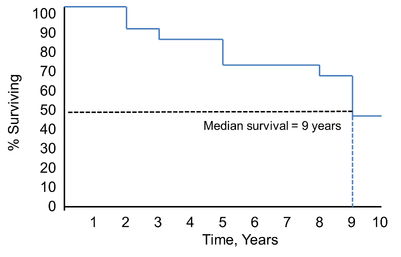
Notice that the survival probability is 100% for 2 years and then drops to 90%. The median survival is 9 years (i.e., 50% of the population survive 9 years; see dashed lines).

Example:

Consider a small prospective cohort study designed to study time to death. The study involves 20 participants who are 65 years of age and older; they are enrolled over a 5 year period and are followed for up to 24 years until they die, the study ends, or they drop out of the study (lost to follow-up). [Note that if a participant enrolls after the study start, their maximum follow up time is less than 24 years. e.g., if a participant enrolls two years after the study start, their maximum follow up time is 22 years.] The data are shown below. In the study, there are 6 deaths and 3 participants with complete follow-up (i.e., 24 years). The remaining 11 have fewer than 24 years of follow-up due to enrolling late or loss to follow-up.

Participant Identification Number	Year of Death	Year of Last Contact
1		24
2	3
3		11
4		19
5		24
6		13
7	14
8		2
9		18
10		17
11		24
12		21
13		12
14	1
15		10
16	23
17		6
18	5
19		9
20	17

 

Life Table (Actuarial Table)

One way of summarizing the experiences of the participants is with a life table, or an actuarial table. Life tables are often used in the insurance industry to estimate life expectancy and to set premiums. We focus on a particular type of life table used widely in biostatistical analysis called a cohort life table or a follow-up life table. The follow-up life table summarizes the experiences of participants over a pre-defined follow-up period in a cohort study or in a clinical trial until the time of the event of interest or the end of the study, whichever comes first.

To construct a life table, we first organize the follow-up times into equally spaced intervals. In the table above we have a maximum follow-up of 24 years, and we consider 5-year intervals (0-4, 5-9, 10-14, 15-19 and 20-24 years). We sum the number of participants who are alive at the beginning of each interval, the number who die, and the number who are censored in each interval. 

Interval in Years	Number Alive at Beginning of Interval	Number of Deaths During Interval	Number Censored
0-4	20	2	1
5-9	17	1	2
10-14	14	1	4
15-19	9	1	3
20-24	5	1	4

We use the following notation in our life table analysis. We first define the notation and then use it to construct the life table.

• N_t = number of participants who are event free and considered at risk during interval t (e.g., in this example the number alive as our outcome of interest is death)
• D_t = number of participants who die (or suffer the event of interest) during interval t
• C_t = number of participants who are censored during interval t N_t* = the average number of participants at risk during interval t
• N_t* = the average number of participants at risk during interval t [In constructing actuarial life tables, the following assumptions are often made: First, the events of interest (e.g., deaths) are assumed to occur at the end of the interval and censored events are assumed to occur uniformly (or evenly) throughout the interval. Therefore, an adjustment is often made to N_t to reflect the average number of participants at risk during the interval, N_t*, which is computed as follows: Nt* =N_t-C_t/2 (i.e., we subtract half of the censored events).
• q_t = proportion dying (or suffering event) during interval t, q_t = D_t/N_t*
• p_t = proportion surviving (remaining event free) interval t, p_t = 1-q_t
• S_t, the proportion surviving (or remaining event free) past interval t; this is sometimes called the cumulative survival probability and it is computed as follows: First, the proportion of participants surviving past time 0 (the starting time) is defined as S₀ = 1 (all participants alive or event free at time zero or study start). The proportion surviving past each subsequent interval is computed using principles of conditional probability introduced in the module on Probability. Specifically, the probability that a participant survives past interval 1 is S₁ = p₁. The probability that a participant survives past interval 2 means that they had to survive past interval 1 and through interval 2: S₂ = P(survive past interval 2) = P(survive through interval 2)*P(survive past interval 1), or S₂ = p₂*S₁. In general, S_t+1 = p_t+1*S_t.

The format of the follow-up life table is shown below.

For the first interval, 0-4 years: At time 0, the start of the first interval (0-4 years), there are 20 participants alive or at risk. Two participants die in the interval and 1 is censored. We apply the correction for the number of participants censored during that interval to produce N_t* =N_t-C_t/2 = 20-(1/2) = 19.5. The computations of the remaining columns are show in the table. The probability that a participant survives past 4 years, or past the first interval (using the upper limit of the interval to define the time) is S₄ = p₄ = 0.897.

For the second interval, 5-9 years: The number at risk is the number at risk in the previous interval (0-4 years) less those who die and are censored (i.e., N_t = N_t-1-D_t-1-C_t-1 = 20-2-1 = 17). The probability that a participant survives past 9 years is S₉ = p₉*S₄ = 0.937*0.897 = 0.840.

 

Interval in Years	Number At Risk During Interval, Nt	Average Number At Risk During Interval, Nt*	Number of Deaths During Interval, Dt	Lost to Follow-Up, Ct	Proportion Dying During Interval, qt	Among Those at Risk, Proportion Surviving Interval, pt	Survival Probability St
0-4	20	20-(1/2) = 19.5	2	1	2/19.5 = 0.103	1-0.103 = 0.897	1(0.897) = 0.897
5-9	17	17-(2/2) = 16.0	1	2	1/16 = 0.063	1-0.063 = 0.937	(0.897)(0.937)=0.840

 

The complete follow-up life table is shown below. 

Interval in Years	Number At Risk During Interval, Nt	Average Number At Risk During Interval, Nt*	Number of Deaths During Interval, Dt	Lost to Follow-Up, Ct	Proportion Dying During Interval, qt	Among Those at Risk, Proportion Surviving Interval, pt	Survival Probability St
0-4	20	19.5	2	1	0.103	0.897	0.897
5-9	17	16.0	1	2	0.063	0.937	0.840
10-14	14	12.0	1	4	0.083	0.917	0.770
15-19	9	7.5	1	3	0.133	0.867	0.668
20-24	5	3.0	1	4	0.333	0.667	0.446

This table uses the actuarial method to construct the follow-up life table where the time is divided into equally spaced intervals.

Kaplan-Meier (Product Limit) Approach

An issue with the life table approach shown above is that the survival probabilities can change depending on how the intervals are organized, particularly with small samples. The Kaplan-Meier approach, also called the product-limit approach, is a popular approach which addresses this issue by re-estimating the survival probability each time an event occurs.

Appropriate use of the Kaplan-Meier approach rests on the assumption that censoring is independent of the likelihood of developing the event of interest and that survival probabilities are comparable in participants who are recruited early and later into the study. When comparing several groups, it is also important that these assumptions are satisfied in each comparison group and that for example, censoring is not more likely in one group than another.

The table below uses the Kaplan-Meier approach to present the same data that was presented above using the life table approach. Note that we start the table with Time=0 and Survival Probability = 1. At Time=0 (baseline, or the start of the study), all participants are at risk and the survival probability is 1 (or 100%). With the Kaplan-Meier approach, the survival probability is computed using S_t+1 = S_t*((N_t+1-D_t+1)/N_t+1). Note that the calculations using the Kaplan-Meier approach are similar to those using the actuarial life table approach. The main difference is the time intervals, i.e., with the actuarial life table approach we consider equally spaced intervals, while with the Kaplan-Meier approach, we use observed event times and censoring times. The calculations of the survival probabilities are detailed in the first few rows of the table.

Life Table Using the Kaplan-Meier Approach

Time, Years	Number at Risk Nt	Number of Deaths Dt	Number Censored Ct	Survival Probability St+1 = St*((Nt+1-Dt+1)/Nt+1)
0	20			1
1	20	1		1*((20-1)/20) = 0.950
2	19		1	0.950*((19-0)/19)=0.950
3	18	1		0.950*((18-1)/18) = 0.897
5	17	1		0.897*((17-1)/17) = 0.844
6	16		1	0.844
9	15		1	0.844
10	14		1	0.844
11	13		1	0.844
12	12		1	0.844
13	11		1	0.844
14	10	1		0.760
17	9	1	1	0.676
18	7		1	0.676
19	6		1	0.676
21	5		1	0.676
23	4	1		0.507
24	3		3	0.507

With large data sets, these computations are tedious. However, these analyses can be generated by statistical computing programs like SAS. Excel can also be used to compute the survival probabilities once the data are organized by times and the numbers of events and censored times are summarized. 

From the life table we can produce a Kaplan-Meier survival curve.

Kaplan-Meier Survival Curve for the Data Above

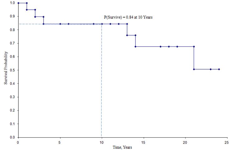
In the survival curve shown above, the symbols represent each event time, either a death or a censored time. From the survival curve, we can also estimate the probability that a participant survives past 10 years by locating 10 years on the X axis and reading up and over to the Y axis. The proportion of participants surviving past 10 years is 84%, and the proportion of participants surviving past 20 years is 68%. The median survival is estimated by locating 0.5 on the Y axis and reading over and down to the X axis. The median survival is approximately 23 years.

Standard Errors and Confidence Interval Estimates of Survival Probabilities

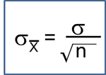
These estimates of survival probabilities at specific times and the median survival time are point estimates and should be interpreted as such. There are formulas to produce standard errors and confidence interval estimates of survival probabilities that can be generated with many statistical computing packages. A popular formula to estimate the standard error of the survival estimates is called Greenwoods⁵ formula and is as follows:

The quantity is summed for numbers at risk (N_t) and numbers of deaths (D_t) occurring through the time of interest (i.e., cumulative, across all times before the time of interest, see example in the table below). Standard errors are computed for the survival estimates for the data in the table below. Note the final column shows the quantity 1.96*SE(S_t) which is the margin of error and used for computing the 95% confidence interval estimates (i.e., S_t ± 1.96 x SE(S_t)). 

Standard Errors of Survival Estimates

Time, Years	Number at Risk Nt	Number of Deaths Dt	Survival Probability St				1.96*SE (St)
0	20		1
1	20	1	0.950	0.003	0.003	0.049	0.096
2	19		0.950	0.000	0.003	0.049	0.096
3	18	1	0.897	0.003	0.006	0.069	0.135
5	17	1	0.844	0.004	0.010	0.083	0.162
6	16		0.844	0.000	0.010	0.083	0.162
9	15		0.844	0.000	0.010	0.083	0.162
10	14		0.844	0.000	0.010	0.083	0.162
11	13		0.844	0.000	0.010	0.083	0.162
12	12		0.844	0.000	0.010	0.083	0.162
13	11		0.844	0.000	0.010	0.083	0.162
14	10	1	0.760	0.011	0.021	0.109	0.214
17	9	1	0.676	0.014	0.035	0.126	0.246
18	7		0.676	0.000	0.035	0.126	0.246
19	6		0.676	0.000	0.035	0.126	0.246
21	5		0.676	0.000	0.035	0.126	0.246
23	4	1	0.507	0.083	0.118	0.174	0.341
24	3		0.507	0.000	0.118	0.174	0.341

 

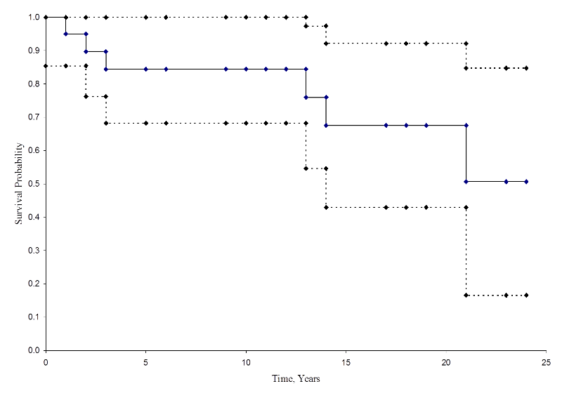
The figure below summarizes the estimates and confidence intervals in the figure below. The Kaplan-Meier survival curve is shown as a solid line, and the 95% confidence limits are shown as dotted lines.

Kaplan-Meier Survival Curve With Confidence Intervals

 

Cumulative Incidence Curves

Some investigators prefer to generate cumulative incidence curves, as opposed to survival curves which show the cumulative probabilities of experiencing the event of interest. Cumulative incidence, or cumulative failure probability, is computed as 1-S_t and can be computed easily from the life table using the Kaplan-Meier approach. The cumulative failure probabilities for the example above are shown in the table below.

Life Table with Cumulative Failure Probabilities

Time, Years	Number at Risk Nt	Number of Deaths Dt	Number Censored Ct	Survival Probability St	Failure Probability 1-St
0	20			1	0
1	20	1		0.950	0.050
2	19		1	0.950	0.050
3	18	1		0.897	0.103
5	17	1		0.844	0.156
6	16		1	0.844	0.156
9	15		1	0.844	0.156
10	14		1	0.844	0.156
11	13		1	0.844	0.156
12	12		1	0.844	0.156
13	11		1	0.844	0.156
14	10	1		0.760	0.240
17	9	1	1	0.676	0.324
18	7		1	0.676	0.324
19	6		1	0.676	0.324
21	5		1	0.676	0.324
23	4	1		0.507	0.493
24	3		3	0.507	0.493

 The figure below shows the cumulative incidence of death for participants enrolled in the study described above. 

Cumulative Incidence Curve

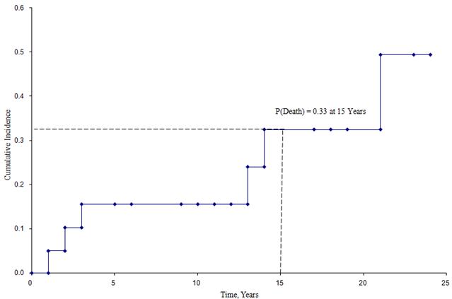
From this figure we can estimate the likelihood that a participant dies by a certain time point. For example, the probability of death is approximately 33% at 15 years (See dashed lines).

return to top | previous page | next page