Survival Analysis

Author:

Lisa Sullivan, PhD

Professor of Biostatistics

Boston University School of Public Health

Introduction

This module introduces statistical techniques to analyze a "time to event outcome variable," which is a different type of outcome variable than those considered in the previous modules. A time to event variable reflects the time until a participant has an event of interest (e.g., heart attack, goes into cancer remission, death). Statistical analysis of time to event variables requires different techniques than those described thus far for other types of outcomes because of the unique features of time to event variables. Statistical analysis of these variables is called time to event analysis or survival analysis even though the outcome is not always death. What we mean by "survival" in this context is remaining free of a particular outcome over time.

The questions of interest in survival analysis are questions like: What is the probability that a participant survives 5 years? Are there differences in survival between groups (e.g., between those assigned to a new versus a standard drug in a clinical trial)? How do certain personal, behavioral or clinical characteristics affect participants' chances of survival?

Learning Objectives

After completing this module, the student will be able to:

1. Identify applications with time to event outcomes
2. Construct a life table using the actuarial approach
3. Construct a life table using the Kaplan-Meier approach
4. Perform and interpret the log rank test
5. Compute and interpret a hazard ratio
6. Interpret coefficients in Cox proportional hazards regression analysis

Time to Event Variables

There are unique features of time to event variables. First, times to event are always positive and their distributions are often skewed. For example, in a study assessing time to relapse in high risk patients, the majority of events (relapses) may occur early in the follow up with very few occurring later. On the other hand, in a study of time to death in a community based sample, the majority of events (deaths) may occur later in the follow up. Standard statistical procedures that assume normality of distributions do not apply. Nonparametric procedures could be invoked except for the fact that there are additional issues. Specifically, complete data (actual time to event data) is not always available on each participant in a study. In many studies, participants are enrolled over a period of time (months or years) and the study ends on a specific calendar date. Thus, participants who enroll later are followed for a shorter period than participants who enroll early. Some participants may drop out of the study before the end of the follow-up period (e.g., move away, become disinterested) and others may die during the follow-up period (assuming the outcome of interest is not death).

In each of these instances, we have incomplete follow-up information. True survival time (sometimes called failure time) is not known because the study ends or because a participant drops out of the study before experiencing the event. What we know is that the participants survival time is greater than their last observed follow-up time. These times are called censored times.

Censoring

There are several different types of censoring. The most common is called right censoring and occurs when a participant does not have the event of interest during the study and thus their last observed follow-up time is less than their time to event. This can occur when a participant drops out before the study ends or when a participant is event free at the end of the observation period.

In the first instance, the participants observed time is less than the length of the follow-up and in the second, the participant's observed time is equal to the length of the follow-up period. These issues are illustrated in the following examples.

Example:

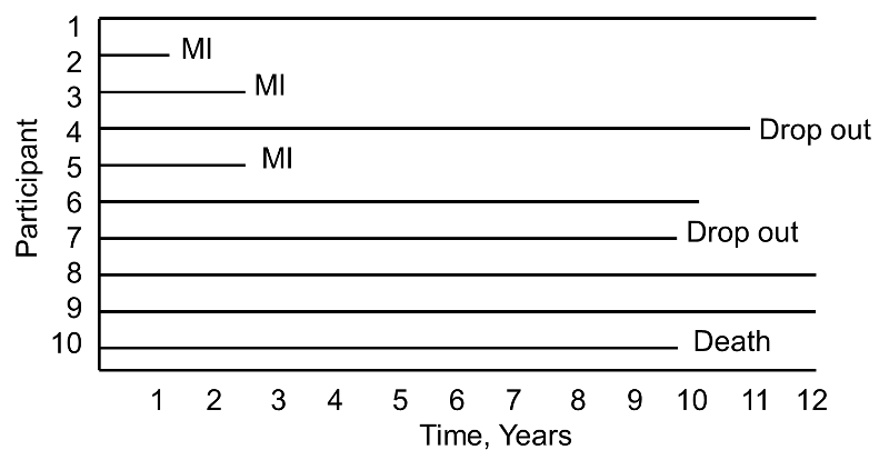
A small prospective study is run and follows ten participants for the development of myocardial infarction (MI, or heart attack) over a period of 10 years. Participants are recruited into the study over a period of two years and are followed for up to 10 years. The graphic below indicates when they enrolled and what subsequently happened to them during the observation period.

During the study period, three participants suffer myocardial infarction (MI), one dies, two drop out of the study (for unknown reasons), and four complete the 10-year follow-up without suffering MI. The figure below shows the same data, but shows survival time starting at a common time zero (i.e., as if all participants enrolled in the study at the same time).

Based on this data, what is the likelihood that a participant will suffer an MI over 10 years? Three of 10 participants suffer MI over the course of follow-up, but 30% is probably an underestimate of the true percentage as two participants dropped out and might have suffered an MI had they been observed for the full 10 years. Their observed times are censored. In addition, one participant dies after 3 years of follow-up. Should these three individuals be included in the analysis, and if so, how?

If we exclude all three, the estimate of the likelihood that a participant suffers an MI is 3/7 = 43%, substantially higher than the initial estimate of 30%. The fact that all participants are often not observed over the entire follow-up period makes survival data unique. In this small example, participant 4 is observed for 4 years and over that period does not have an MI. Participant 7 is observed for 2 years and over that period does not have an MI. While they do not suffer the event of interest, they contribute important information. Survival analysis techniques make use of this information in the estimate of the probability of event.

 Now consider the same study and the experiences of 10 different participants as depicted below.

Notice here that, once again, three participants suffer MI, one dies, two drop out of the study, and four complete the 10-year follow-up without suffering MI. However, the events (MIs) occur much earlier, and the drop outs and death occur later in the course of follow-up. Should these differences in participants experiences affect the estimate of the likelihood that a participant suffers an MI over 10 years?

In survival analysis we analyze not only the numbers of participants who suffer the event of interest (a dichotomous indicator of event status), but also the times at which the events occur.

Introduction to Survival Data

Survival analysis focuses on two important pieces of information:

1. Whether or not a participant suffers the event of interest during the study period (i.e., a dichotomous or indicator variable often coded as 1=event occurred or 0=event did not occur during the study observation period.
2. The follow up time for each individual being followed.

Follow Up Time

Time zero, or the time origin, is the time at which participants are considered at-risk for the outcome of interest. In many studies, time at risk is measured from the start of the study (i.e., at enrollment). In a prospective cohort study evaluating time to incident stroke, investigators may recruit participants who are 55 years of age and older as the risk for stroke prior to that age is very low. In a prospective cohort study evaluating time to incident cardiovascular disease, investigators may recruit participants who are 35 years of age and older. In each of these studies, a minimum age might be specified as a criterion for inclusion in the study. Follow up time is measured from time zero (the start of the study or from the point at which the participant is considered to be at risk) until the event occurs, the study ends or the participant is lost, whichever comes first. In a clinical trial, the time origin is usually considered the time of randomization. Patients often enter or are recruited into cohort studies and clinical trials over a period of several calendar months or years. Thus, it is important to record the entry time so that the follow up time is accurately measured. Again, our interest lies in the time to event but for various reasons (e.g., the participant drops out of the study or the study observation period ends) we cannot always measure time to event. For participants who do not suffer the event of interest we measure follow up time which is less than time to event, and these follow up times are censored.

The Survival Function

In survival analysis, we use information on event status and follow up time to estimate a survival function. Consider a 20 year prospective study of patient survival following a myocardial infarction. In this study, the outcome is all-cause mortality and the survival function (or survival curve) might be as depicted in the figure below.

Sample Survival Curve - Probability Of Surviving

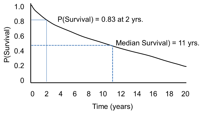
The horizontal axis represents time in years, and the vertical axis shows the probability of surviving or the proportion of people surviving.

• At time zero, the survival probability is 1.0 (or 100% of the participants are alive).
• At 2 years, the probability of survival is approximately 0.83 or 83%.
• At 10 years, the probability of survival is approximately 0.55 or 55%.
• The median survival is approximately 11 years.

A flat survival curve (i.e. one that stays close to 1.0) suggests very good survival, whereas a survival curve that drops sharply toward 0 suggests poor survival.

The figure above shows the survival function as a smooth curve. In most applications, the survival function is shown as a step function rather than a smooth curve (see the next page.)

The figure below shows Kaplan-Meier curves for the cumulative risk of dementia among elderly persons who frequently played board games such as chess, checkers, backgammon, or cards at baseline as compared with subjects who rarely played such games.

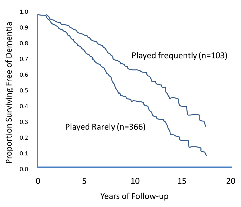
Source: Adapted from Verghese et al.

Estimating the Survival Function

There are several different ways to estimate a survival function or a survival curve. There are a number of popular parametric methods that are used to model survival data, and they differ in terms of the assumptions that are made about the distribution of survival times in the population. Some popular distributions include the exponential, Weibull, Gompertz and log-normal distributions.² Perhaps the most popular is the exponential distribution, which assumes that a participant's likelihood of suffering the event of interest is independent of how long that person has been event-free. Other distributions make different assumptions about the probability of an individual developing an event (i.e., it may increase, decrease or change over time). More details on parametric methods for survival analysis can be found in Hosmer and Lemeshow and Lee and Wang^1,3.

We focus here on two nonparametric methods, which make no assumptions about how the probability that a person develops the event changes over time. Using nonparametric methods, we estimate and plot the survival distribution or the survival curve. Survival curves are often plotted as step functions, as shown in the figure below. Time is shown on the X-axis and survival (proportion of people at risk) is shown on the Y-axis. Note that the percentage of participants surviving does not always represent the percentage who are alive (which assumes that the outcome of interest is death). "Survival" can also refer to the proportion who are free of another outcome event (e.g., percentage free of MI or cardiovascular disease), or it can also represent the percentage who do not experience a healthy outcome (e.g., cancer remission).

Survival Function

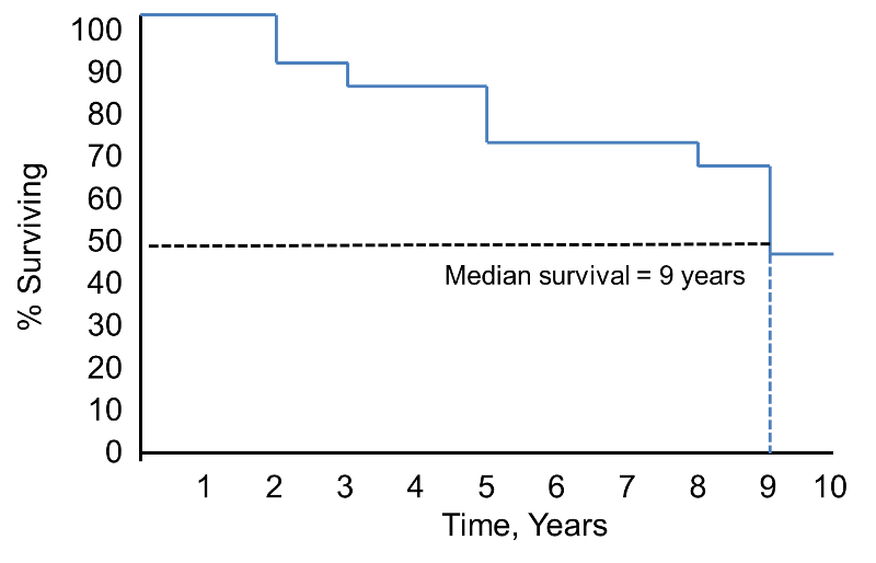
Notice that the survival probability is 100% for 2 years and then drops to 90%. The median survival is 9 years (i.e., 50% of the population survive 9 years; see dashed lines).

Example:

Consider a small prospective cohort study designed to study time to death. The study involves 20 participants who are 65 years of age and older; they are enrolled over a 5 year period and are followed for up to 24 years until they die, the study ends, or they drop out of the study (lost to follow-up). [Note that if a participant enrolls after the study start, their maximum follow up time is less than 24 years. e.g., if a participant enrolls two years after the study start, their maximum follow up time is 22 years.] The data are shown below. In the study, there are 6 deaths and 3 participants with complete follow-up (i.e., 24 years). The remaining 11 have fewer than 24 years of follow-up due to enrolling late or loss to follow-up.

Life Table (Actuarial Table)

One way of summarizing the experiences of the participants is with a life table, or an actuarial table. Life tables are often used in the insurance industry to estimate life expectancy and to set premiums. We focus on a particular type of life table used widely in biostatistical analysis called a cohort life table or a follow-up life table. The follow-up life table summarizes the experiences of participants over a pre-defined follow-up period in a cohort study or in a clinical trial until the time of the event of interest or the end of the study, whichever comes first.

To construct a life table, we first organize the follow-up times into equally spaced intervals. In the table above we have a maximum follow-up of 24 years, and we consider 5-year intervals (0-4, 5-9, 10-14, 15-19 and 20-24 years). We sum the number of participants who are alive at the beginning of each interval, the number who die, and the number who are censored in each interval. 

We use the following notation in our life table analysis. We first define the notation and then use it to construct the life table.

• N_t = number of participants who are event free and considered at risk during interval t (e.g., in this example the number alive as our outcome of interest is death)
• D_t = number of participants who die (or suffer the event of interest) during interval t
• C_t = number of participants who are censored during interval t N_t* = the average number of participants at risk during interval t
• N_t* = the average number of participants at risk during interval t [In constructing actuarial life tables, the following assumptions are often made: First, the events of interest (e.g., deaths) are assumed to occur at the end of the interval and censored events are assumed to occur uniformly (or evenly) throughout the interval. Therefore, an adjustment is often made to N_t to reflect the average number of participants at risk during the interval, N_t*, which is computed as follows: Nt* =N_t-C_t/2 (i.e., we subtract half of the censored events).
• q_t = proportion dying (or suffering event) during interval t, q_t = D_t/N_t*
• p_t = proportion surviving (remaining event free) interval t, p_t = 1-q_t
• S_t, the proportion surviving (or remaining event free) past interval t; this is sometimes called the cumulative survival probability and it is computed as follows: First, the proportion of participants surviving past time 0 (the starting time) is defined as S₀ = 1 (all participants alive or event free at time zero or study start). The proportion surviving past each subsequent interval is computed using principles of conditional probability introduced in the module on Probability. Specifically, the probability that a participant survives past interval 1 is S₁ = p₁. The probability that a participant survives past interval 2 means that they had to survive past interval 1 and through interval 2: S₂ = P(survive past interval 2) = P(survive through interval 2)*P(survive past interval 1), or S₂ = p₂*S₁. In general, S_t+1 = p_t+1*S_t.

The format of the follow-up life table is shown below.

For the first interval, 0-4 years: At time 0, the start of the first interval (0-4 years), there are 20 participants alive or at risk. Two participants die in the interval and 1 is censored. We apply the correction for the number of participants censored during that interval to produce N_t* =N_t-C_t/2 = 20-(1/2) = 19.5. The computations of the remaining columns are show in the table. The probability that a participant survives past 4 years, or past the first interval (using the upper limit of the interval to define the time) is S₄ = p₄ = 0.897.

For the second interval, 5-9 years: The number at risk is the number at risk in the previous interval (0-4 years) less those who die and are censored (i.e., N_t = N_t-1-D_t-1-C_t-1 = 20-2-1 = 17). The probability that a participant survives past 9 years is S₉ = p₉*S₄ = 0.937*0.897 = 0.840.

The complete follow-up life table is shown below. 

This table uses the actuarial method to construct the follow-up life table where the time is divided into equally spaced intervals.

Kaplan-Meier (Product Limit) Approach

An issue with the life table approach shown above is that the survival probabilities can change depending on how the intervals are organized, particularly with small samples. The Kaplan-Meier approach, also called the product-limit approach, is a popular approach which addresses this issue by re-estimating the survival probability each time an event occurs.

Appropriate use of the Kaplan-Meier approach rests on the assumption that censoring is independent of the likelihood of developing the event of interest and that survival probabilities are comparable in participants who are recruited early and later into the study. When comparing several groups, it is also important that these assumptions are satisfied in each comparison group and that for example, censoring is not more likely in one group than another.

The table below uses the Kaplan-Meier approach to present the same data that was presented above using the life table approach. Note that we start the table with Time=0 and Survival Probability = 1. At Time=0 (baseline, or the start of the study), all participants are at risk and the survival probability is 1 (or 100%). With the Kaplan-Meier approach, the survival probability is computed using S_t+1 = S_t*((N_t+1-D_t+1)/N_t+1). Note that the calculations using the Kaplan-Meier approach are similar to those using the actuarial life table approach. The main difference is the time intervals, i.e., with the actuarial life table approach we consider equally spaced intervals, while with the Kaplan-Meier approach, we use observed event times and censoring times. The calculations of the survival probabilities are detailed in the first few rows of the table.

Life Table Using the Kaplan-Meier Approach

With large data sets, these computations are tedious. However, these analyses can be generated by statistical computing programs like SAS. Excel can also be used to compute the survival probabilities once the data are organized by times and the numbers of events and censored times are summarized. 

From the life table we can produce a Kaplan-Meier survival curve.

Kaplan-Meier Survival Curve for the Data Above

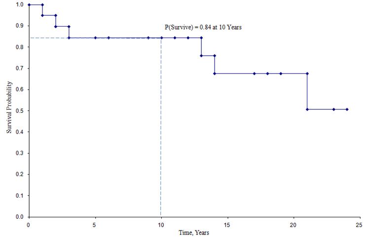
In the survival curve shown above, the symbols represent each event time, either a death or a censored time. From the survival curve, we can also estimate the probability that a participant survives past 10 years by locating 10 years on the X axis and reading up and over to the Y axis. The proportion of participants surviving past 10 years is 84%, and the proportion of participants surviving past 20 years is 68%. The median survival is estimated by locating 0.5 on the Y axis and reading over and down to the X axis. The median survival is approximately 23 years.

Standard Errors and Confidence Interval Estimates of Survival Probabilities

These estimates of survival probabilities at specific times and the median survival time are point estimates and should be interpreted as such. There are formulas to produce standard errors and confidence interval estimates of survival probabilities that can be generated with many statistical computing packages. A popular formula to estimate the standard error of the survival estimates is called Greenwoods⁵ formula and is as follows:

The quantity is summed for numbers at risk (N_t) and numbers of deaths (D_t) occurring through the time of interest (i.e., cumulative, across all times before the time of interest, see example in the table below). Standard errors are computed for the survival estimates for the data in the table below. Note the final column shows the quantity 1.96*SE(S_t) which is the margin of error and used for computing the 95% confidence interval estimates (i.e., S_t ± 1.96 x SE(S_t)). 

Standard Errors of Survival Estimates

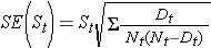
The figure below summarizes the estimates and confidence intervals in the figure below. The Kaplan-Meier survival curve is shown as a solid line, and the 95% confidence limits are shown as dotted lines.

Kaplan-Meier Survival Curve With Confidence Intervals

Cumulative Incidence Curves

Some investigators prefer to generate cumulative incidence curves, as opposed to survival curves which show the cumulative probabilities of experiencing the event of interest. Cumulative incidence, or cumulative failure probability, is computed as 1-S_t and can be computed easily from the life table using the Kaplan-Meier approach. The cumulative failure probabilities for the example above are shown in the table below.

Life Table with Cumulative Failure Probabilities

 The figure below shows the cumulative incidence of death for participants enrolled in the study described above. 

Cumulative Incidence Curve

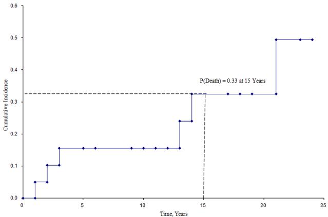
From this figure we can estimate the likelihood that a participant dies by a certain time point. For example, the probability of death is approximately 33% at 15 years (See dashed lines).

Comparing Survival Curves

We are often interested in assessing whether there are differences in survival (or cumulative incidence of event) among different groups of participants. For example, in a clinical trial with a survival outcome, we might be interested in comparing survival between participants receiving a new drug as compared to a placebo (or standard therapy). In an observational study, we might be interested in comparing survival between men and women, or between participants with and without a particular risk factor (e.g., hypertension or diabetes). There are several tests available to compare survival among independent groups.

The Log Rank Test

The log rank test is a popular test to test the null hypothesis of no difference in survival between two or more independent groups. The test compares the entire survival experience between groups and can be thought of as a test of whether the survival curves are identical (overlapping) or not. Survival curves are estimated for each group, considered separately, using the Kaplan-Meier method and compared statistically using the log rank test. It is important to note that there are several variations of the log rank test statistic that are implemented by various statistical computing packages (e.g., SAS, R ^4,6). We present one version here that is linked closely to the chi-square test statistic and compares observed to expected numbers of events at each time point over the follow-up period.

Example:

A small clinical trial is run to compare two combination treatments in patients with advanced gastric cancer. Twenty participants with stage IV gastric cancer who consent to participate in the trial are randomly assigned to receive chemotherapy before surgery or chemotherapy after surgery. The primary outcome is death and participants are followed for up to 48 months (4 years) following enrollment into the trial. The experiences of participants in each arm of the trial are shown below.

Six participants in the chemotherapy before surgery group die over the course of follow-up as compared to three participants in the chemotherapy after surgery group. Other participants in each group are followed for varying numbers of months, some to the end of the study at 48 months (in the chemotherapy after surgery group). Using the procedures outlined above, we first construct life tables for each treatment group using the Kaplan-Meier approach.

Life Table for Group Receiving Chemotherapy Before Surgery

Life Table for Group Receiving Chemotherapy After Surgery

The two survival curves are shown below.

Survival in Each Treatment Group

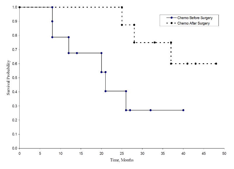
The survival probabilities for the chemotherapy after surgery group are higher than the survival probabilities for the chemotherapy before surgery group, suggesting a survival benefit. However, these survival curves are estimated from small samples. To compare survival between groups we can use the log rank test. The null hypothesis is that there is no difference in survival between the two groups or that there is no difference between the populations in the probability of death at any point. The log rank test is a non-parametric test and makes no assumptions about the survival distributions. In essence, the log rank test compares the observed number of events in each group to what would be expected if the null hypothesis were true (i.e., if the survival curves were identical).

H₀: The two survival curves are identical (or S_1t = S_2t) versus H₁: The two survival curves are not identical (or S_1t ≠ S_2t, at any time t) (α=0.05).

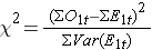
The log rank statistic is approximately distributed as a chi-square test statistic. There are several forms of the test statistic, and they vary in terms of how they are computed. We use the following:

where ΣO_jt represents the sum of the observed number of events in the j^th group over time (e.g., j=1,2) and ΣE_jt represents the sum of the expected number of events in the jth group over time.

The sums of the observed and expected numbers of events are computed for each event time and summed for each comparison group. The log rank statistic has degrees of freedom equal to k-1, where k represents the number of comparison groups. In this example, k=2 so the test statistic has 1 degree of freedom.

To compute the test statistic we need the observed and expected number of events at each event time. The observed number of events are from the sample and the expected number of events are computed assuming that the null hypothesis is true (i.e., that the survival curves are identical).

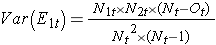
To generate the expected numbers of events we organize the data into a life table with rows representing each event time, regardless of the group in which the event occurred. We also keep track of group assignment. We then estimate the proportion of events that occur at each time (O_t/N_t) using data from both groups combined under the assumption of no difference in survival (i.e., assuming the null hypothesis is true). We multiply these estimates by the number of participants at risk at that time in each of the comparison groups (N_1t and N_2t for groups 1 and 2 respectively).

Specifically, we compute for each event time t, the number at risk in each group, N_jt (e.g., where j indicates the group, j=1, 2) and the number of events (deaths), O_jt ,in each group. The table below contains the information needed to conduct the log rank test to compare the survival curves above. Group 1 represents the chemotherapy before surgery group, and group 2 represents the chemotherapy after surgery group.

Data for Log Rank Test to Compare Survival Curves

 We next total the number at risk, N_t = N_1t+N_2t, at each event time and the number of observed events (deaths), O_t = O_1t+O_2t, at each event time. We then compute the expected number of events in each group. The expected number of events is computed at each event time as follows:

E_1t = N_1t*(O_t/N_t) for group 1 and E_2t = N_2t*(O_t/N_t) for group 2. The calculations are shown in the table below.

Expected Numbers of Events in Each Group

 We next sum the observed numbers of events in each group (∑O_1t and ΣO_2t) and the expected numbers of events in each group (ΣE_1t and ΣE_2t) over time. These are shown in the bottom row of the next table below.

Total Observed and Expected Numbers of Observed in each Group

 We can now compute the test statistic:

The test statistic is approximately distributed as chi-square with 1 degree of freedom. Thus, the critical value for the test can be found in the table of Critical Values of the Χ² Distribution.

For this test the decision rule is to Reject H₀ if Χ² > 3.84. We observe Χ² = 6.151, which exceeds the critical value of 3.84. Therefore, we reject H₀. We have significant evidence, α=0.05, to show that the two survival curves are different. 

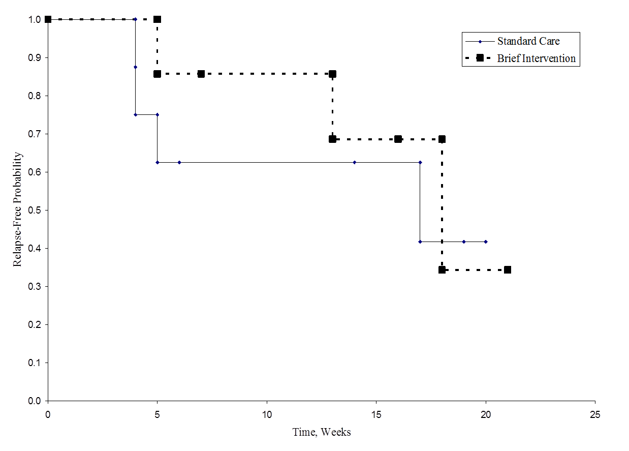
Example:

An investigator wishes to evaluate the efficacy of a brief intervention to prevent alcohol consumption in pregnancy. Pregnant women with a history of heavy alcohol consumption are recruited into the study and randomized to receive either the brief intervention focused on abstinence from alcohol or standard prenatal care. The outcome of interest is relapse to drinking. Women are recruited into the study at approximately 18 weeks gestation and followed through the course of pregnancy to delivery (approximately 39 weeks gestation). The data are shown below and indicate whether women relapse to drinking and if so, the time of their first drink measured in the number of weeks from randomization. For women who do not relapse, we record the number of weeks from randomization that they are alcohol free.

The question of interest is whether there is a difference in time to relapse between women assigned to standard prenatal care as compared to those assigned to the brief intervention.

• Step 1.

Set up hypotheses and determine level of significance.

H₀: Relapse-free time is identical between groups versus

H₁: Relapse-free time is not identical between groups (α=0.05)

• Step 2.

Select the appropriate test statistic.

The test statistic for the log rank test is

• Step 3.

Set up the decision rule.

The test statistic follows a chi-square distribution, and so we find the critical value in the table of critical values for the Χ² distribution) for df=k-1=2-1=1 and α=0.05. The critical value is 3.84 and the decision rule is to reject H₀ if Χ² > 3.84. 

• Step 4.

Compute the test statistic.

To compute the test statistic, we organize the data according to event (relapse) times and determine the numbers of women at risk in each treatment group and the number who relapse at each observed relapse time. In the following table, group 1 represents women who receive standard prenatal care and group 2 represents women who receive the brief intervention. 

We next total the number at risk, , at each event time, the number of observed events (relapses), , at each event time and determine the expected number of relapses in each group at each event time using and .

We then sum the observed numbers of events in each group (ΣO_1t and ΣO_2t) and the expected numbers of events in each group (ΣE_1t and ΣE_2t) over time. The calculations for the data in this example are shown below. 

We now compute the test statistic:

• Step 5.

Conclusion. Do not reject H₀ because 0.726 < 3.84. We do not have statistically significant evidence at α=0.05, to show that the time to relapse is different between groups.

 The figure below shows the survival (relapse-free time) in each group. Notice that the survival curves do not show much separation, consistent with the non-significant findings in the test of hypothesis.

Relapse-Free Time in Each Group

As noted, there are several variations of the log rank statistic. Some statistical computing packages use the following test statistic for the log rank test to compare two independent groups:

where ΣO_1t is the sum of the observed number of events in group 1, and ΣE_1t is the sum of the expected number of events in group 1 taken over all event times. The denominator is the sum of the variances of the expected numbers of events at each event time, which is computed as follows:

There are other versions of the log rank statistic as well as other tests to compare survival functions between independent groups.^7-9 For example, a popular test is the modified Wilcoxon test which is sensitive to larger differences in hazards earlier as opposed to later in follow-up.¹⁰ 

Cox Proportional Hazards Regression Analysis

Survival analysis methods can also be extended to assess several risk factors simultaneously similar to multiple linear and multiple logistic regression analysis as described in the modules discussing Confounding, Effect Modification, Correlation, and Multivariable Methods. One of the most popular regression techniques for survival analysis is Cox proportional hazards regression, which is used to relate several risk factors or exposures, considered simultaneously, to survival time. In a Cox proportional hazards regression model, the measure of effect is the hazard rate, which is the risk of failure (i.e., the risk or probability of suffering the event of interest), given that the participant has survived up to a specific time. A probability must lie in the range 0 to 1. However, the hazard represents the expected number of events per one unit of time. As a result, the hazard in a group can exceed 1. For example, if the hazard is 0.2 at time t and the time units are months, then on average, 0.2 events are expected per person at risk per month. Another interpretation is based on the reciprocal of the hazard. For example, 1/0.2 = 5, which is the expected event-free time (5 months) per person at risk.

 In most situations, we are interested in comparing groups with respect to their hazards, and we use a hazard ratio, which is analogous to an odds ratio in the setting of multiple logistic regression analysis. The hazard ratio can be estimated from the data we organize to conduct the log rank test. Specifically, the hazard ratio is the ratio of the total number of observed to expected events in two independent comparison groups:

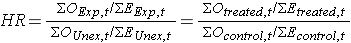
In some studies, the distinction between the exposed or treated as compared to the unexposed or control groups are clear. In other studies, it is not. In the latter case, either group can appear in the numerator and the interpretation of the hazard ratio is then the risk of event in the group in the numerator as compared to the risk of event in the group in the denominator.

In Example 3 there are two active treatments being compared (chemotherapy before surgery versus chemotherapy after surgery). Consequently, it does not matter which appears in the numerator of the hazard ratio. Using the data in Example 3, the hazard ratio is estimated as:

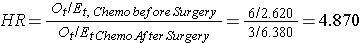
Thus, the risk of death is 4.870 times higher in the chemotherapy before surgery group as compared to the chemotherapy after surgery group.

Example 3 examined the association of a single independent variable (chemotherapy before or after surgery) on survival. However, it is often of interest to assess the association between several risk factors, considered simultaneously, and survival time. One of the most popular regression techniques for survival outcomes is Cox proportional hazards regression analysis. There are several important assumptions for appropriate use of the Cox proportional hazards regression model, including

1. independence of survival times between distinct individuals in the sample,
2. a multiplicative relationship between the predictors and the hazard (as opposed to a linear one as was the case with multiple linear regression analysis, discussed in more detail below), and
3. a constant hazard ratio over time.

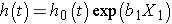
The Cox proportional hazards regression model can be written as follows:

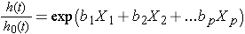
where h(t) is the expected hazard at time t, h₀(t) is the baseline hazard and represents the hazard when all of the predictors (or independent variables) X₁, X₂ , X_p are equal to zero. Notice that the predicted hazard (i.e., h(t)), or the rate of suffering the event of interest in the next instant, is the product of the baseline hazard (h₀(t)) and the exponential function of the linear combination of the predictors. Thus, the predictors have a multiplicative or proportional effect on the predicted hazard.

Consider a simple model with one predictor, X₁. The Cox proportional hazards model is:

Suppose we wish to compare two participants in terms of their expected hazards, and the first has X₁= a and the second has X₁= b. The expected hazards are h(t) = h₀(t)exp (b_1a) and h(t) = h₀(t)exp (b_1b), respectively.

The hazard ratio is the ratio of these two expected hazards: h₀(t)exp (b_1a)/ h₀(t)exp (b_1b) = exp(b_1(a-b)) which does not depend on time, t. Thus the hazard is proportional over time.

Sometimes the model is expressed differently, relating the relative hazard, which is the ratio of the hazard at time t to the baseline hazard, to the risk factors:

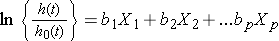
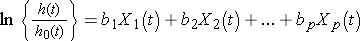
We can take the natural logarithm (ln) of each side of the Cox proportional hazards regression model, to produce the following which relates the log of the relative hazard to a linear function of the predictors. Notice that the right hand side of the equation looks like the more familiar linear combination of the predictors or risk factors (as seen in the multiple linear regression model).

In practice, interest lies in the associations between each of the risk factors or predictors (X₁, X₂, ..., X_p) and the outcome. The associations are quantified by the regression coefficients coefficients (b₁, b₂, ..., b_p). The technique for estimating the regression coefficients in a Cox proportional hazards regression model is beyond the scope of this text and is described in Cox and Oakes.⁹ Here we focus on interpretation. The estimated coefficients in the Cox proportional hazards regression model, b₁, for example, represent the change in the expected log of the hazard ratio relative to a one unit change in X₁, holding all other predictors constant.

The antilog of an estimated regression coefficient, exp(b_i), produces a hazard ratio. If a predictor is dichotomous (e.g., X₁ is an indicator of prevalent cardiovascular disease or male sex) then exp(b₁) is the hazard ratio comparing the risk of event for participants with X₁=1 (e.g., prevalent cardiovascular disease or male sex) to participants with X₁=0 (e.g., free of cardiovascular disease or female sex).

If the hazard ratio for a predictor is close to 1 then that predictor does not affect survival. If the hazard ratio is less than 1, then the predictor is protective (i.e., associated with improved survival) and if the hazard ratio is greater than 1, then the predictor is associated with increased risk (or decreased survival).

Tests of hypothesis are used to assess whether there are statistically significant associations between predictors and time to event. The examples that follow illustrate these tests and their interpretation.

The Cox proportional hazards model is called a semi-parametric model, because there are no assumptions about the shape of the baseline hazard function. There are however, other assumptions as noted above (i.e., independence, changes in predictors produce proportional changes in the hazard regardless of time, and a linear association between the natural logarithm of the relative hazard and the predictors). There are other regression models used in survival analysis that assume specific distributions for the survival times such as the exponential, Weibull, Gompertz and log-normal distributions^1,8. The exponential regression survival model, for example, assumes that the hazard function is constant. Other distributions assume that the hazard is increasing over time, decreasing over time, or increasing initially and then decreasing. Example 5 will illustrate estimation of a Cox proportional hazards regression model and discuss the interpretation of the regression coefficients.

Example:

An analysis is conducted to investigate differences in all-cause mortality between men and women participating in the Framingham Heart Study adjusting for age. A total of 5,180 participants aged 45 years and older are followed until time of death or up to 10 years, whichever comes first. Forty six percent of the sample are male, the mean age of the sample is 56.8 years (standard deviation = 8.0 years) and the ages range from 45 to 82 years at the start of the study. There are a total of 402 deaths observed among 5,180 participants. Descriptive statistics are shown below on the age and sex of participants at the start of the study classified by whether they die or do not die during the follow up period.

We now estimate a Cox proportional hazards regression model and relate an indicator of male sex and age, in years, to time to death. The parameter estimates are generated in SAS using the SAS Cox proportional hazards regression procedure¹² and are shown below along with their p-values. 

Note that there is a positive association between age and all-cause mortality and between male sex and all-cause mortality (i.e., there is increased risk of death for older participants and for men).

Again, the parameter estimates represent the increase in the expected log of the relative hazard for each one unit increase in the predictor, holding other predictors constant. There is a 0.11149 unit increase in the expected log of the relative hazard for each one year increase in age, holding sex constant, and a 0.67958 unit increase in expected log of the relative hazard for men as compared to women, holding age constant.

For interpretability, we compute hazard ratios by exponentiating the parameter estimates. For age, exp(0.11149) = 1.118. There is an 11.8% increase in the expected hazard relative to a one year increase in age (or the expected hazard is 1.12 times higher in a person who is one year older than another), holding sex constant. Similarly, exp(0.67958) = 1.973. The expected hazard is 1.973 times higher in men as compared to women, holding age constant.

Suppose we consider additional risk factors for all-cause mortality and estimate a Cox proportional hazards regression model relating an expanded set of risk factors to time to death. The parameter estimates are again generated in SAS using the SAS Cox proportional hazards regression procedure and are shown below along with their p-values.¹² Also included below are the hazard ratios along with their 95% confidence intervals.

All of the parameter estimates are estimated taking the other predictors into account. After accounting for age, sex, blood pressure and smoking status, there are no statistically significant associations between total serum cholesterol and all-cause mortality or between diabetes and all-cause mortality. This is not to say that these risk factors are not associated with all-cause mortality; their lack of significance is likely due to confounding (interrelationships among the risk factors considered). Notice that for the statistically significant risk factors (i.e., age, sex, systolic blood pressure and current smoking status), that the 95% confidence intervals for the hazard ratios do not include 1 (the null value). In contrast, the 95% confidence intervals for the non-significant risk factors (total serum cholesterol and diabetes) include the null value.

Example:

A prospective cohort study is run to assess the association between body mass index and time to incident cardiovascular disease (CVD). At baseline, participants' body mass index is measured along with other known clinical risk factors for cardiovascular disease (e.g., age, sex, blood pressure). Participants are followed for up to 10 years for the development of CVD. In the study of n=3,937 participants, 543 develop CVD during the study observation period. In a Cox proportional hazards regression analysis, we find the association between BMI and time to CVD statistically significant with a parameter estimate of 0.02312 (p=0.0175) relative to a one unit change in BMI.

If we exponentiate the parameter estimate, we have a hazard ratio of 1.023 with a confidence interval of (1.004-1.043). Because we model BMI as a continuous predictor, the interpretation of the hazard ratio for CVD is relative to a one unit change in BMI (recall BMI is measured as the ratio of weight in kilograms to height in meters squared). A one unit increase in BMI is associated with a 2.3% increase in the expected hazard.

To facilitate interpretation, suppose we create 3 categories of weight defined by participant's BMI.

• Normal weight is defined as BMI < 25.0,
• Overweight as BMI between 25.0 and 29.9, and
• Obese as BMI exceeding 29.9.

In the sample, there are 1,651 (42%) participants who meet the definition of normal weight, 1,648 (42%) who meet the definition of over weight, and 638 (16%) who meet the definition of obese. The numbers of CVD events in each of the 3 groups are shown below.

The incidence of CVD is higher in participants classified as overweight and obese as compared to participants of normal weight.

We now use Cox proportional hazards regression analysis to make maximum use of the data on all participants in the study. The following table displays the parameter estimates, p-values, hazard ratios and 95% confidence intervals for the hazards ratios when we consider the weight groups alone (unadjusted model), when we adjust for age and sex and when we adjust for age, sex and other known clinical risk factors for incident CVD.

The latter two models are multivariable models and are performed to assess the association between weight and incident CVD adjusting for confounders. Because we have three weight groups, we need two dummy variables or indicator variables to represent the three groups. In the models we include the indicators for overweight and obese and consider normal weight the reference group.

 * Adjusted for age, sex, systolic blood pressure, treatment for hypertension, current smoking status, total serum cholesterol.

 In the unadjusted model, there is an increased risk of CVD in overweight participants as compared to normal weight and in obese as compared to normal weight participants (hazard ratios of 1.215 and 1.310, respectively). However, after adjustment for age and sex, there is no statistically significant difference between overweight and normal weight participants in terms of CVD risk (hazard ratio = 1.067, p=0.5038). The same is true in the model adjusting for age, sex and the clinical risk factors. However, after adjustment, the difference in CVD risk between obese and normal weight participants remains statistically significant, with approximately a 30% increase in risk of CVD among obese participants as compared to participants of normal weight.

Extensions

There are a number of important extensions of the approach that are beyond the scope of this text.

Time-Dependent Covariates

In the previous examples, we considered the effect of risk factors measured at the beginning of the study period, or at baseline, but there are many applications where the risk factors or predictors change over time. Suppose we wish to assess the impact of exposure to nicotine and alcohol during pregnancy on time to preterm delivery. Smoking and alcohol consumption may change during the course of pregnancy. These predictors are called time-dependent covariates and they can be incorporated into survival analysis models. The Cox proportional hazards regression model with time dependent covariates takes the form:

Notice that each of the predictors, X₁, X₂, ... , X_p, now has a time component. There are also many predictors, such as sex and race, that are independent of time. Survival analysis models can include both time dependent and time independent predictors simultaneously. Many statistical computing packages (e.g., SAS¹²) offer options for the inclusion of time dependent covariates. A difficult aspect of the analysis of time-dependent covariates is the appropriate measurement and management of these data for inclusion in the models.

Proportionality Assumption 

A very important assumption for the appropriate use of the log rank test and the Cox proportional hazards regression model is the proportionality assumption.

Specifically, we assume that the hazards are proportional over time which implies that the effect of a risk factor is constant over time. There are several approaches to assess the proportionality assumption, some are based on statistical tests and others involve graphical assessments.

In the statistical testing approach, predictor by time interaction effects are included in the model and tested for statistical significance. If one (or more) of the predictor by time interactions reaches statistical significance (e.g., p<0.05), then the assumption of proportionality is violated. An alternative approach to assessing proportionality is through graphical analysis. There are several graphical displays that can be used to assess whether the proportional hazards assumption is reasonable. These are often based on residuals and examine trends (or lack thereof) over time. More details can be found in Hosmer and Lemeshow¹.

If either a statistical test or a graphical analysis suggest that the hazards are not proportional over time, then the Cox proportional hazards model is not appropriate, and adjustments must be made to account for non-proportionality. One approach is to stratify the data into groups such that within groups the hazards are proportional, and different baseline hazards are estimated in each stratum (as opposed to a single baseline hazard as was the case for the model presented earlier). Many statistical computing packages offer this option.

Competing Risks

The competing risks issue is one in which there are several possible outcome events of interest. For example, a prospective study may be conducted to assess risk factors for time to incident cardiovascular disease. Cardiovascular disease includes myocardial infarction, coronary heart disease, coronary insufficiency and many other conditions. The investigator measures whether each of the component outcomes occurs during the study observation period as well as the time to each distinct event. The goal of the analysis is to determine the risk factors for each specific outcome and the outcomes are correlated. Interested readers should see Kalbfleisch and Prentice¹⁰ for more details.

Summary

Time to event data, or survival data, are frequently measured in studies of important medical and public health issues. Because of the unique features of survival data, most specifically the presence of censoring, special statistical procedures are necessary to analyze these data. In survival analysis applications, it is often of interest to estimate the survival function, or survival probabilities over time. There are several techniques available; we present here two popular nonparametric techniques called the life table or actuarial table approach and the Kaplan-Meier approach to constructing cohort life tables or follow-up life tables. Both approaches generate estimates of the survival function which can be used to estimate the probability that a participant survives to a specific time (e.g., 5 or 10 years).

The notation and template for each approach are summarized below.

 Actuarial, Follow-Up Life Table Approach

Kaplan-Meier Approach

It is often of interest to assess whether there are statistically significant differences in survival between groups between competing treatment groups in a clinical trial or between men and women, or patients with and without a specific risk factor in an observational study. There are many statistical tests available; we present the log rank test, which is a popular non-parametric test. It makes no assumptions about the survival distributions and can be conducted relatively easily using life tables based on the Kaplan-Meier approach.

There are several variations of the log rank statistic as well as other tests to compare survival curves between independent groups.

We use the following test statistic which is distributed as a chi-square statistic with degrees of freedom k-1, where k represents the number of independent comparison groups:

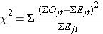
where ΣO_jt represents the sum of the observed number of events in the jth group over time and ΣE_jt represents the sum of the expected number of events in the jth group over time. The observed and expected numbers of events are computed for each event time and summed for each comparison group over time. To compute the log rank test statistic, we compute for each event time t, the number at risk in each group, N_jt (e.g., where j indicates the group) and the observed number of events O_jt in each group. We then sum the number at risk, N_t , in each group over time to produce ΣN_jt , the number of observed events O_t , in each group over time to produce ΣO_jt , and compute the expected number of events in each group using E_jt = N_jt*(O_t/N_t) at each time. The expected numbers of events are then summed over time to produce ΣE_jt for each group.

Finally, there are many applications in which it is of interest to estimate the effect of several risk factors, considered simultaneously, on survival. Cox proportional hazards regression analysis is a popular multivariable technique for this purpose. The Cox proportional hazards regression model is as follows:

where h(t) is the expected hazard at time t, h0(t) is the baseline hazard and represents the hazard when all of the predictors X_1,   X₂ ... , X_p are equal to zero.

The associations between risk factors and survival time in a Cox proportional hazards model are often summarized by hazard ratios. The hazard ratio for a dichotomous risk factor (e.g., treatment assignment in a clinical trial or prevalent diabetes in an observational study) represents the increase or decrease in the hazard in one group as compared to the other.

For example, in a clinical trial with survival time as the outcome, if the hazard ratio is 0.5 comparing participants on a treatment to those on placebo, this suggests a 50% reduction in the hazard (risk of failure assuming the person survived to a certain point) in the treatment group as compared to the placebo. In an observational study with survival time as the outcome, if the hazard ratio is 1.25 comparing participants with prevalent diabetes to those free of diabetes then the risk of failure is 25% higher in participants with diabetes.

References

1. Hosmer, DW and Lemeshow, S. Applied Survival Analysis: Regression Modeling of Time to Event Data. NewYork: John Wiley and Sons; 1999.
2. Cox DR, Oakes D. Analysis of Survival Data, Chapman and Hall, 1984.
3. Lee ET and Wang JW. Statistical Methods for Survival Data Analysis. 3rd edition. New York: John Wiley & Sons; 2003.
4. SAS version 9.1© 2002-2003 by SAS Institute, Inc., Cary, NC. 
5. Greenwood M, Jr. The Natural Duration of Cancer. Reports of Public Health and Related Subjects Vol 33, HMSO, London; 1926.
6. Crawley MJ. Statistics: An Introduction using R. NewYork: John Wiley and Sons; 2005.
7. Mantel, N. Evaluation of survival data and two new rank order statistics arising in its consideration. Cancer Chemotherapy Reports. 1966; 50 (3): 163- 70.
8. Peto R and Peto J. Asymptotically Efficient Rank Invariant Test Procedures. Journal of the Royal Statistical Society. Series A (General). 1972; 135 (2): 185-207.
9. Gehan EA. A Generalized Wilcoxon Test for Comparing Arbitrarily Singly-Censored Samples. Biometrika. 1965; 52: 203-223.
10. Kalbfleisch JD and Prentice RL. The Statistical Analysis of Failure Time Data. 2nd ed. New York: Wiley, 2002.
11. Kleinbaun DG and Klein M. Survival Analysis: A Self-Learning Text. New York: Springer Science + Business Median, Inc., 2005.
12. Allison P. Survival Analysis Using the SAS System, SAS Institute, 1995.