


Parameter Estimation
There are a number of population parameters of potential interest when one is estimating health outcomes (or "endpoints"). Many of the outcomes we are interested in estimating are either continuous or dichotomous variables, although there are other types which are discussed in a later module. The parameters to be estimated depend not only on whether the endpoint is continuous or dichotomous, but also on the number of groups being studied. Moreover, when two groups are being compared, it is important to establish whether the groups are independent (e.g., men versus women) or dependent (i.e., matched or paired, such as a before and after comparison). The table below summarizes parameters that may be important to estimate in health-related studies.
|
|
Parameters Being Estimated |
|
|---|---|---|
|
|
Continuous Variable |
Dichotomous Variable |
|
One Sample |
mean |
proportion or rate, e.g., prevalence, cumulative incidence, incidence rate |
|
Two Independent Samples |
difference in means |
difference in proportions or rates, e.g., risk difference, rate difference, risk ratio, odds ratio, attributable proportion |
|
Two Dependent, Matched Samples |
mean difference |
|
Confidence Intervals
There are two types of estimates for each population parameter: the point estimate and confidence interval (CI) estimate. For both continuous variables (e.g., population mean) and dichotomous variables (e.g., population proportion) one first computes the point estimate from a sample. Recall that sample means and sample proportions are unbiased estimates of the corresponding population parameters.
For both continuous and dichotomous variables, the confidence interval estimate (CI) is a range of likely values for the population parameter based on:
- the point estimate, e.g., the sample mean
- the investigator's desired level of confidence (most commonly 95%, but any level between 0-100% can be selected)
- and the sampling variability or the standard error of the point estimate.
Strictly speaking a 95% confidence interval means that if we were to take 100 different samples and compute a 95% confidence interval for each sample, then approximately 95 of the 100 confidence intervals will contain the true mean value (μ). In practice, however, we select one random sample and generate one confidence interval, which may or may not contain the true mean. The observed interval may over- or underestimate μ. Consequently, the 95% CI is the likely range of the true, unknown parameter. The confidence interval does not reflect the variability in the unknown parameter. Rather, it reflects the amount of random error in the sample and provides a range of values that are likely to include the unknown parameter. Another way of thinking about a confidence interval is that it is the range of likely values of the parameter (defined as the point estimate + margin of error) with a specified level of confidence (which is similar to a probability).
Suppose we want to generate a 95% confidence interval estimate for an unknown population mean. This means that there is a 95% probability that the confidence interval will contain the true population mean. Thus, P( [sample mean] - margin of error < μ < [sample mean] + margin of error) = 0.95.
The Central Limit Theorem introduced in the module on Probability stated that, for large samples, the distribution of the sample means is approximately normally distributed with a mean:

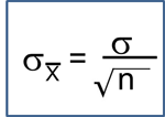
and a standard deviation (also called the standard error):
For the standard normal distribution, P(-1.96 < Z < 1.96) = 0.95, i.e., there is a 95% probability that a standard normal variable, Z, will fall between -1.96 and 1.96. The Central Limit Theorem states that for large samples:
By substituting the expression on the right side of the equation:
Using algebra, we can rework this inequality such that the mean (μ) is the middle term, as shown below.

then
and finally
This last expression, then, provides the 95% confidence interval for the population mean, and this can also be expressed as:
Thus, the margin of error is 1.96 times the standard error (the standard deviation of the point estimate from the sample), and 1.96 reflects the fact that a 95% confidence level was selected. So, the general form of a confidence interval is:
point estimate + Z SE (point estimate)
where Z is the value from the standard normal distribution for the selected confidence level (e.g., for a 95% confidence level, Z=1.96).
In practice, we often do not know the value of the population standard deviation (σ). However, if the sample size is large (n > 30), then the sample standard deviations can be used to estimate the population standard deviation.
Table - Z-Scores for Commonly Used Confidence Intervals
|
Desired Confidence Interval |
Z Score |
|
90% 95% 99% |
1.645 1.96 2.576 |

In the health-related publications a 95% confidence interval is most often used, but this is an arbitrary value, and other confidence levels can be selected. Note that for a given sample, the 99% confidence interval would be wider than the 95% confidence interval, because it allows one to be more confident that the unknown population parameter is contained within the interval.
Confidence Interval Estimates for Smaller Samples
With smaller samples (n< 30) the Central Limit Theorem does not apply, and another distribution called the t distribution must be used. The t distribution is similar to the standard normal distribution but takes a slightly different shape depending on the sample size. In a sense, one could think of the t distribution as a family of distributions for smaller samples. Instead of "Z" values, there are "t" values for confidence intervals which are larger for smaller samples, producing larger margins of error, because small samples are less precise. t values are listed by degrees of freedom (df). Just as with large samples, the t distribution assumes that the outcome of interest is approximately normally distributed.
A table of t values is shown in the frame below. Note that the table can also be accessed from the "Other Resources" on the right side of the page.
![]()