


Control Selection Bias in a Case-Control Study
The Key to Understanding Selection Bias
In all of the mechanisms that result in selection bias, there is over or under representation of one or more of the exposure-disease categories, i.e., one or more of the cells in the contingency table over or under represents what is true in the source population. As a result, the sample is not representative of the source population, and the estimate of association will be biased - either over-estimated or under-estimated.
|
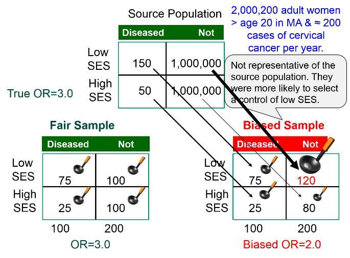
Suppose we wish to study the possible association between socioeconomic status (SES), defined based on current household income) and risk of cancer of the cervix. We have a source population with 2,000,200 women in whom there are 200 cases of cancer of the cervix during a calendar year.
If we studied all women in the source population and simply used the median household income to classify them as "higher" or "lower" SES, we would have found the exposure-disease distribution in the table below.
|
|
Cervical Cancer |
No Cancer |
|
Lower SES |
150 |
1,000,000 |
|
Higher SES |
50 |
1,000,000 |
The risk ratio and the odds ratio are both 3.0
However, we can't study the entire population, and since the outcome is relatively uncommon, we decide to do a case-control study. We begin by going to a large medical center that treats cervical cancer patients who are referred from all over the state and identify 100 patients with cervical cancer who agree to be interviewed. The interviews reveal that 75 of the women are from households with incomes that meet our definition of lower SES, and the other 25 are higher SES. To get non-disease control subjects, we send members of our research team into the neighborhood around the medical center and have them go door to door during the day to invite women to be interviewed as controls for our study. In many cases, no one seems to be home, but our team persists and eventually finds 200 control women, of whom 120 meet our definition of lower SES, and 80 who are of higher SES. The sample we have selected is summarized in the contingency table below, which is oriented to facilitate the use of the oddsratio.wald function in R.
|
|
No Cancer |
Cancer |
|
Higher SES (ref) |
80 |
25 |
|
Lower SES |
120 |
75 |
The analysis is performed as follows:
> ORtable<-matrix(c(80,120,25,75),nrow = 2,ncol = 2)
> oddsratio.wald(ORtable)
$data
Outcome
Predictor Disease1 Disease2 Total
Exposed1 80 25 105
Exposed2 120 75 195
Total 200 100 300
$measure
odds ratio with 95% C.I.
Predictor estimate lower upper
Exposed1 1 NA NA
Exposed2 2 1.172783 3.410692
$p.value
two-sided
Predictor midp.exact fisher.exact chi.square
Exposed1 NA NA NA
Exposed2 0.009913739 0.01048725 0.01023571
To summarize, the estimated odds ratio was 2.0; the 95% confidence interval for the odds ratio was 1.17 to 3.41; and the p-value was 0.01.
The result is statistically significant, but the estimated measure of association is biased. The odds ratio in the source population was 3.0, but the odds ratio in the biased sample was 2.0, i.e., there was bias toward the null. What went wrong?
The estimated OR was biased because counts in the contingency table for the sample were not representative of the exposure-disease distribution in the source population, which was the entire state. The cases, who were referred from all over the state did, in fact, indicate the exposure distribution in diseased women in the source population, i.e. 75 to 25 or 3:1. However, the exposure distribution among the 200 controls in the sample (120:80) was not representative of the exposure distribution in non-disease women in the source population (1:1). This occurred because the controls were selected by a different mechanism. By going door to door during working hours, the research team missed many women who were employed, so the sample over-selected women who were unemployed. Therefore, there was a greater tendency to select non-diseased controls of lower SES.
|
The key thing to remember here is that one of the four cells in my contingency table was over-sampled (and one was under sampled).
|
The figure below summarizes this scenario, showing the distribution in the source population at the top, the contingency table for the biased sample at the lower right, and the contingency table from a fair sample at the lower left. We have used images of ladles to represent the relative sampling for the contingency tables at the bottom. The representative sample has ladles in each of the four cells that are of equal size indicating a proportionate sample that is representative of the distributions in the source population. However, the biased sample at the lower right has a larger ladle for the non-diseased controls of lower SES, who were over-sampled because of the enrollment method used for the controls, and the controls of higher SES were therefore under sampled, as shown by a smaller ladle.
Rules for Avoiding Selection Bias in a Case-Control Study
- Controls must come from the same source population as the cases and must be representative of the exposure distribution in the source population. One way to test whether the controls have been selected appropriately is to consider the "would criterion," i.e., if the controls had experienced the outcome, would they have been identified as potential cases? If not, there is selection bias.
- Controls must be selected independently from exposure, meaning that whether or not a person is exposed or unexposed should not influence selection or enrollment of a control subject.
 Test Yourself
Hemifacial microsomia is a rare congenital malformation in which the lower half of one side of the face is underdeveloped and does not grow normally. The condition varies in severity and is sometimes subtle and only recognized by an astute pediatrician. Affected children can be referred for surgery to improve facial symmetry by reconstructing the bony and soft tissues, but the surgery is only done in certain large medical centers that receive referrals from all over the United States.
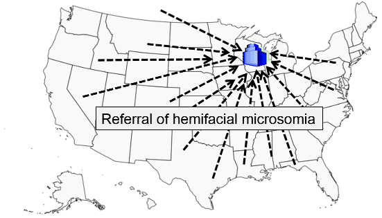
Researchers wanted to study whether maternal smoking or maternal diabetes are associated with the risk of this condition in their offspring. The names of children treated for this problem were obtained from a medical center in Michigan that specializes in this type of corrective surgery. How can they identify control subjects in a way that avoids selection bias? [Hint: How can they ensure that the "would criterion" is met?] Think about this for a few minutes, and try to devise an unbiased sampling strategy for controls before you look at how the investigators achieved this.
