PH717 Module 10 - Bias
Identifying and Preventing Bias

Introduction

 We have already alluded to sources of error in epidemiologic studies, and you have learned a number of methods for evaluating random error. We will now turn our attention to biases, i.e., systematic errors that are usually unwittingly introduced into a study by the investigators or the subjects that cause an over- or under-estimate of an association between an exposure and a health outcome.

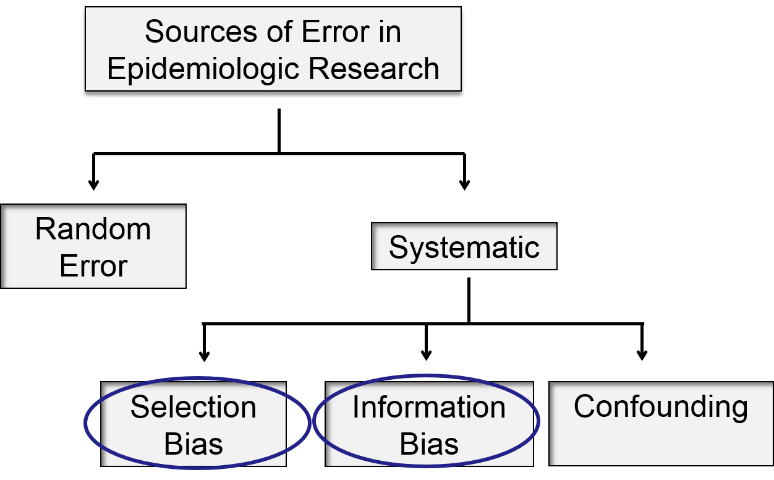
In this module we will focus on selection bias and information bias.

• Selection bias occurs when the participants selected into a study or who happen to be retained during a longitudinal study are not representative of the source population, because their selection or retention was related to their exposure-disease status.
• Information bias occurs if there are errors in classifying participants with regard to their exposure status or their outcome status.

By identifying common mechanisms of bias, we can design studies to limit these pitfalls, predict the impact of bias on our study results, and critically evaluate the published literature.

Essential Questions:

1. What systematic errors in population health research can lead to incorrect conclusions?
2. Why do these errors occur? Are they specific to certain study designs?
3. What is selection bias and information bias?
4. How can we estimate the effect of bias on my findings? How can we avoid or minimize these errors?

Learning Objectives

After completing this module, you will be able to:

• Define bias (systematic error) and differentiate between random error and systematic error
• Describe selection bias and identify why and how it occurs in different study designs
• Describe ways to minimize the effect of selection bias
• Define information bias and identify why and how it occurs
• Determine whether a particular bias in a given study would result in an overestimate or an underestimate of the strength of association, i.e., whether the bias is toward the nul or away from the null.
• Evaluate data to determine whether bias is likely to have occurred in a given study
• Identify which types of studies are prone to particular types of bias
• Identify common sources of bias and strategies to prevent selection and information bias

Control Selection Bias in a Case-Control Study

The Key to Understanding Selection Bias   In all of the mechanisms that result in selection bias, there is over or under representation of one or more of the exposure-disease categories, i.e., one or more of the cells in the contingency table over or under represents what is true in the source population. As a result, the sample is not representative of the source population, and the estimate of association will be biased - either over-estimated or under-estimated.

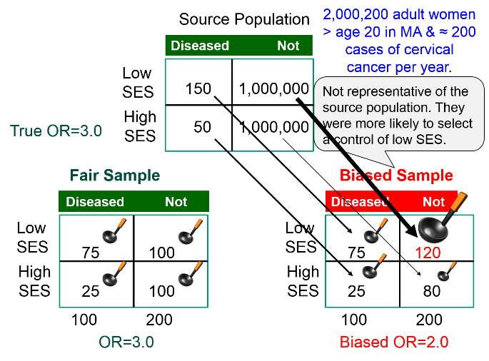
Suppose we wish to study the possible association between socioeconomic status (SES), defined based on current household income) and risk of cancer of the cervix. We have a source population with 2,000,200 women in whom there are 200 cases of cancer of the cervix during a calendar year.

If we studied all women in the source population and simply used the median household income to classify them as "higher" or "lower" SES,   we would have found the exposure-disease distribution in the table below.

The risk ratio and the odds ratio are both 3.0

However, we can't study the entire population, and since the outcome is relatively uncommon, we decide to do a case-control study. We begin by going to a large medical center that treats cervical cancer patients who are referred from all over the state and identify 100 patients with cervical cancer who agree to be interviewed. The interviews reveal that 75 of the women are from households with incomes that meet our definition of lower SES, and the other 25 are higher SES. To get non-disease control subjects, we send members of our research team into the neighborhood around the medical center and have them go door to door during the day to invite women to be interviewed as controls for our study. In many cases, no one seems to be home, but our team persists and eventually finds 200 control women, of whom 120 meet our definition of lower SES, and 80 who are of higher SES. The sample we have selected is summarized in the contingency table below, which is oriented to facilitate the use of the oddsratio.wald function in R.

The analysis is performed as follows:

> ORtable<-matrix(c(80,120,25,75),nrow = 2,ncol = 2)
> oddsratio.wald(ORtable)

$data
                  Outcome

Predictor   Disease1 Disease2 Total

  Exposed1       80       25    105
  Exposed2       120       75    195
  Total          200     100    300

$measure

                  odds ratio with 95% C.I.
Predictor   estimate   lower   upper
  Exposed1         1       NA    NA          
  Exposed2         2 1.172783 3.410692

$p.value
                  two-sided
Predictor     midp.exact fisher.exact chi.square
  Exposed1       NA NA NA
Exposed2 0.009913739   0.01048725 0.01023571

To summarize, the estimated odds ratio was 2.0; the 95% confidence interval for the odds ratio was 1.17 to 3.41; and the p-value was 0.01.

The result is statistically significant, but the estimated measure of association is biased. The odds ratio in the source population was 3.0, but the odds ratio in the biased sample was 2.0, i.e., there was bias toward the null. What went wrong?

The estimated OR was biased because counts in the contingency table for the sample were not representative of the exposure-disease distribution in the source population, which was the entire state. The cases, who were referred from all over the state did, in fact, indicate the exposure distribution in diseased women in the source population, i.e. 75 to 25 or 3:1. However, the exposure distribution among the 200 controls in the sample (120:80) was not representative of the exposure distribution in non-disease women in the source population (1:1). This occurred because the controls were selected by a different mechanism. By going door to door during working hours, the research team missed many women who were employed, so the sample over-selected women who were unemployed. Therefore, there was a greater tendency to select non-diseased controls of lower SES.

The figure below summarizes this scenario, showing the distribution in the source population at the top, the contingency table for the biased sample at the lower right, and the contingency table from a fair sample at the lower left. We have used images of ladles to represent the relative sampling for the contingency tables at the bottom. The representative sample has ladles in each of the four cells that are of equal size indicating a proportionate sample that is representative of the distributions in the source population. However, the biased sample at the lower right has a larger ladle for the non-diseased controls of lower SES, who were over-sampled because of the enrollment method used for the controls, and the controls of higher SES were therefore under sampled, as shown by a smaller ladle.

Rules for Avoiding Selection Bias in a Case-Control Study

1. Controls must come from the same source population as the cases and must be representative of the exposure distribution in the source population. One way to test whether the controls have been selected appropriately is to consider the "would criterion," i.e., if the controls had experienced the outcome, would they have been identified as potential cases? If not, there is selection bias.
2. Controls must be selected independently from exposure, meaning that whether or not a person is exposed or unexposed should not influence selection or enrollment of a control subject.

Test Yourself

Hemifacial microsomia is a rare congenital malformation in which the lower half of one side of the face is underdeveloped and does not grow normally. The condition varies in severity and is sometimes subtle and only recognized by an astute pediatrician. Affected children can be referred for surgery to improve facial symmetry by reconstructing the bony and soft tissues, but the surgery is only done in certain large medical centers that receive referrals from all over the United States.

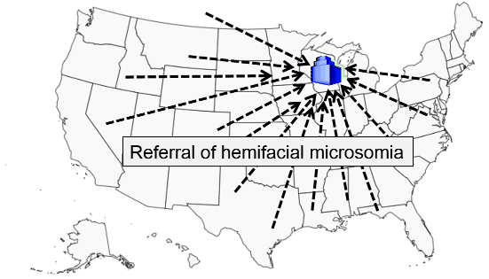
Researchers wanted to study whether maternal smoking or maternal diabetes are associated with the risk of this condition in their offspring. The names of children treated for this problem were obtained from a medical center in Michigan that specializes in this type of corrective surgery. How can they identify control subjects in a way that avoids selection bias? [Hint: How can they ensure that the "would criterion" is met?] Think about this for a few minutes, and try to devise an unbiased sampling strategy for controls before you look at how the investigators achieved this.

Answer

Self-Selection Bias in a Case-Control Study

Selection bias can be introduced into case-control studies with low response or participation rates if the likelihood of responding or participating is related to both the exposure and outcome.

Example:

A case-control study explored an association between family history of heart disease (exposure) and the presence of heart disease in subjects. Volunteers for "a study on heart disease" were recruited from an HMO, but what if subjects with heart disease were more likely to participate if they had a family history of heart disease? If a random selection of 1,000 members of the HMO had been invited to participate and all of them did, then the true odds ratio would have been 2.25 based on the counts in the first table below.

Therefore, the true OR= (3/2)/(2/3) = 2.25

However, suppose the response rates were only 60%, except for those with CHD and a family history, who might have been more likely to participate since they were curious about whether there was an association. Once again, the observed frequencies, shown in the next table, would not have reflected the distribution in the source population, and the resulting odds ratio would be biased.

The biased OR = (240/120)/(120/180) = 3.0

The only was to avoid this type of bias is to achieve high participation rates. The closer one gets to 100% participation, the less likely it is that this bias will affect the results. Participation of 80% or more of those invited is usually sufficient.

Self-selection Bias Occurs Only if Participation is Differential for a Particular Exposure-Disease Cell

If participation is different by exposure status, but not by disease status, the result is not biased. We can illustrate this using the example above in which the unbiased OR = 2.25.

Here, the participation differed between the two exposure categories, but within each exposure category participation was similar for the cases and the controls. As a result, the OR=2.25 (not biased).

Similarly, if participation differs by disease status, but not by exposure status, the result will not be biased.

 Here, the participation differed between the two outcome categories, but within each outcome category participation was similar for the exposure groups. As a result, the OR=2.25 (not biased).

Test Yourself

Researchers conducted a case-control study to determine whether maternal use of anti-depressant medications during pregnancy was associated with a higher risk congenital heart defects in their offspring. Mothers who recently had a baby are asked to participate in the study, and they were told what the research hypothesis was.

Could there be selection bias here? Think about this before looking at the answer below.

Answer

Selection Bias in Cohort Studies and Clinical Trials

Prospective Cohort Studies and Clinical Trials

In the previous examples selection bias occurred because selection or enrollment procedures resulted in over- or under-representation of one or more of the exposure-disease categories. Since prospective cohort studies enroll subjects who have not yet developed the health outcomes of interest, selection bias due to enrollment procedures is rare, but can occur. In addition, prospective cohort studies can have selection bias as a result of differential retention during follow up.

Blood clots that form in the deep veins in the leg can break loose from the venous system and be carried back to the right side of the heart and then to the pulmonary artery where they become lodged and disrupt pulmonary circulation. This is referred to as pulmonary thromboembolism. It is a serious and sometimes fatal event, and some oral contraceptives (OC) have been shown to increase the risk of thrombosis (clot formation in the veins), particularly in older formulations of oral contraceptives.

Consider a hypothetical prospective cohort study of the association between use of oral contraceptives (OC) and development of pulmonary thromboembolism (TE) in women of child-bearing age, as summarized in the figure below. The contingency table at the top shows what the results would have been if there had been complete follow up. There are 10,000 subjects in each group, and 20 out of 10,000 OC users developed TE compared to 10 out of 10,000 women who did not use OC, so the true RR=2.0.

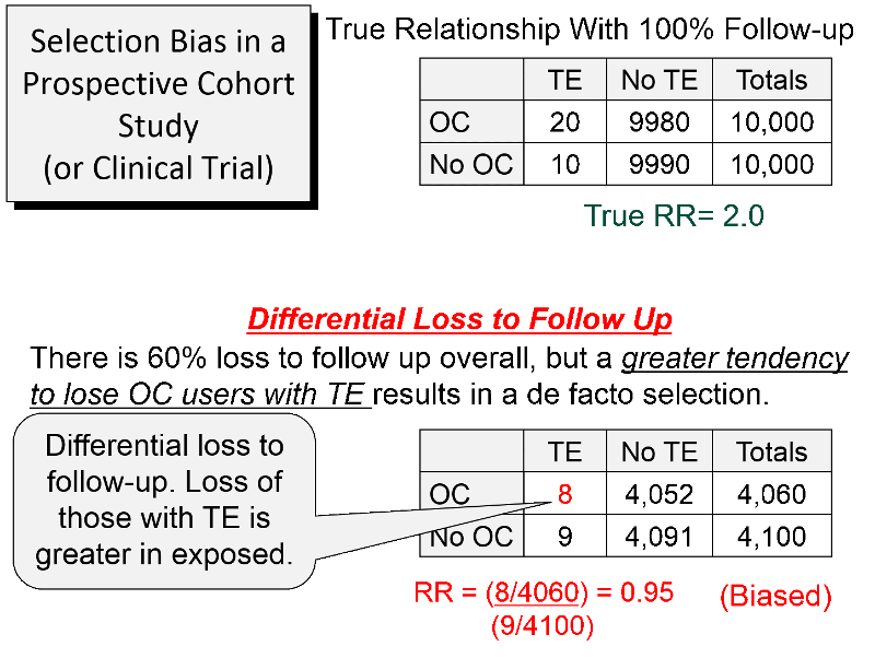
About 60% of the subjects were lost to follow up, as shown in the lower portion of the figure. However, there was differential loss to follow up, since 12 out the 20 women with TE were lost in the OC groups, but only one out of the 10 women with TE in the group not using OCs were lost. In the case-control study discussed above there was over-representation in one of the cells of the table, but here there is under-representation because of greater loss to follow up in women who had both the exposure and the outcome of interest. So, in this prospective cohort study, the sample that is available for analysis is not representative of the source population of women of child-bearing age. The result is a biased estimate from the sample which gives RR=0.95, suggesting no association, even though there is a two-fold increase in risk.

This form of selection bias (bias from differential loss to follow up) can occur in both prospective cohort studies and clinical trials if there are substantial losses to follow up. There is no way of knowing whether loss to follow up is differential, but if follow up rates are greater than 80%, the effects of this form are selection bias are likely to be minimal. The only way to avoid this type of bias is for investigators to do whatever they can to maintain high rates of follow up. If loss to follow up is much greater than 20%, one needs to be increasingly concerned that the estimate might be biased.

Selection Bias in Retrospective Cohort Studies

In a retrospective cohort study selection bias occurs if selection of either exposed or non-exposed subjects is somehow related to the outcome. For example, if researchers are more likely to enroll an exposed person if they have the outcome of interest, the measure of association will be biased.

Example:
Researchers wanted to conduct a retrospective cohort study on the health effects of an occupational exposure to an organic solvent in a factory using employee health records. The truth is that those exposed to the solvent had a two-fold increase in liver damage, and if they had had all of the records, the contingency table would have looked like the table below.

RR= (100/1,000)/(50/1,000) = 2.0

Unfortunately, many of the employee records had been lost or destroyed over the past 20 years. However, there had been suspicions about the health effects of the solvent for many years, and the records of employees who had been exposed and developed health problems were more likely to have been retained. Records were available for 98% of the employees who had been exposed and developed liver damage, but for all other employees only 80% of the records could be found. As a result, the contingency table looked like this.

RR= (98/818)/(40/800) = 2.4

Here, the source population consisted of the employees of the factory, and once again, the data in the sample was not representative of the source population. Specifically, one exposure-disease category had greater retention of records than the others, so the measure of association was biased. In a sense, loss of records in this retrospective cohort study is analogous to differential loss to follow up in prospective cohort studies and clinical trials.

The Health Worker Effect

The general population is sometimes used as a non-exposed comparison group in occupational studies of mortality, since data is readily available, and the general population is mostly unexposed to rare occupational exposures. The main disadvantage is that an employed work force tends to be generally healthier than the general population, because the general population also includes people who cannot work due to disease or disability. Consequently, the risk ratio for death will tend to be underestimated, when the higher risk general population is used as a surrogate for an unexposed work force; this is called "the healthy worker effect". Here, the source population is an employed work force, and death rates in the general population are not necessarily indicative of death rates in an unexposed work force. 

Example:

Suppose an employed work force with a particular occupational exposure has an age-adjusted death rate of 130 per 100,000 workers, and the age-adjusted death rate in a very comparable employed work force that was unexposed was 100 per 100,000. In other words, the true risk ratio is 1.3.

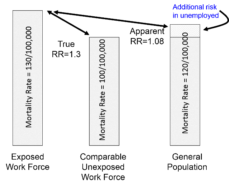
However, the age-adjusted death rate in the general population (which is mostly unexposed to rare occupational exposures) would tend to be higher than that of an unexposed work force, perhaps 120 per 100,000 because of a wide variety of illnesses and disabilities. Using the general population as surrogate for an unexposed work force would result in a risk ratio of 130/120 = 1.08, i.e., an underestimate of the true magnitude of association. 

Summary of Selection Bias

Selection bias occurs when selection, enrollment, or retention of subjects is differential for one of the exposure-disease categories. This can occur in any of the analytic studies, and it can cause either an overestimate or an underestimate of the measure of association.

In case-control studies selection bias can occur due to:

1. Control selection bias: Selection of a comparison group ("controls") that is not representative of the population that produced the cases in a case-control study.
2. Self-selection bias: Refusal, non-response, or agreement to participate that is related to the exposure and disease status.

In cohort studies selection bias can occur due to:

3. The "healthy worker" effect, which tends to cause an underestimate of the association, since death rates in the general population are usually higher than in an employed work force, i.e., the general population is not representative of the source population.
4. Differential loss to follow up can cause an overestimate or an underestimate of effect in retrospective and prospective cohort studies and in clinical trials.

Information Bias

Information bias occurs as a result of misclassification of exposure or disease status. The figure below shows a two-by-two contingency table in which smiley-face icons represent the findings instead of numbers. Subjects who truly have the health outcome of interest are shown with red icons, while those who truly did not develop the outcome are shown with blue icons. Subjects who have the exposure have a thick black outline, while the unexposed subjects do not. Based on this scheme it is apparent that most subjects are in the correct cell of the contingency table, but there are some who have been misclassified and are in an incorrect cell.

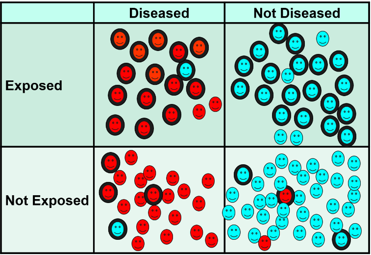
There are some non-diseased people who ended up in the diseased column, and there are some diseased people who were misclassified as non-diseased. In addition, some of those who were exposed were misclassified as unexposed, and some of the unexposed were misclassified as having been exposed. In general, misclassification of this type tends to be more of a problem for exposure status, but outcomes can be misclassified as well.

There are several mechanisms that produce misclassification, and the effects depend on the circumstances. The key distinction is whether the errors in classification are differential or non-differential with respect to the comparison groups.

Non-Differential Misclassification of Exposure

Non-differential misclassification means that the percentage of errors is about equal in the two groups being compared. If there really is an association, non-differential misclassification tends to make the groups appear more similar than they really are, and it causes an underestimate of the association, i.e., "bias toward the null".

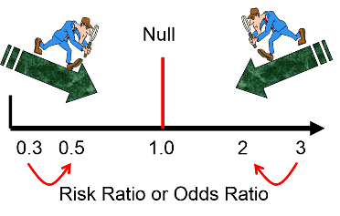
If the true risk ratio or odds ratio is 3, the biased estimate might be 2, and if the true risk ratio or odds ratio is 0.3, the biased estimate might be 0.5. In other words, regardless of whether the effect is an increase in risk or a decrease, non-differential misclassification moves the biased estimate toward the null value.

Mechanisms for Non-differential Misclassification

1. Equally inaccurate memory of exposures in both groups. For example, in a case-control study of heart disease and past activity subjects have difficulty accurately remembering their exercise frequency, duration and intensity over many years. Note that in this scenario cases and controls are equally likely to report their past exercise levels inaccurately. If one group remembers better than the other, it will cause recall bias, which is differential. See Differential Misclassification in the next section.
2. Recording and coding errors in records and databases. For example, many hospitals, insurance companies, and other agencies use codes for exposures, procedures, and diagnoses, such as the ICD-11 system (International Classification of Disease).
3. Using surrogate measures of exposure. For example, using prescriptions for anti-hypertensive medications as an indication that the patient filled the prescription and actually took it regularly is often inaccurate.
4. Non-specific or broad definitions of exposure or outcome. For example, if you are studying the effects of environmental tobacco smoke (ETS) exposure, asking whether a subject's spouse smokes will not capture where, when, and how often they smoke in the subject's presence or the subject's exposure to other sources of ETS, such as in the work place or other venues.

Example:
A case-control study used the diagnostic codes in a state-wide data base of hospital discharge data to estimate the association between diabetes and risk of coronary heart disease (CHD). The table below shows what the true association was.

True OR= (40/10) / (60/90) = 6.0

However, diabetes was under-reported by about 50% in the computerized data base, and the collected data collected looked like this:

Biased OR = (20/5) / (80/95) = 4.75

Differential Misclassification

Differential misclassification occurs when data is more accurate in one of the comparison groups. Depending on the circumstances, differential misclassification can cause either an under-estimate or an over-estimate of the association. There are several mechanisms by which differential misclassification can occur.

Recall Bias

Recall bias occurs when subjects in one of the compared groups recall past exposures more accurately than the other group. This is particularly a problem in case-control studies. Consider a case-control study by Louik et al. whose goal was to determine whether maternal use of anti-depressant medications during pregnancy is associated with an increased risk of congenital defects in the offspring. The use of anti-depressants during pregnancy was determined by interviewing mothers of children with congenital heart defects and mothers of normal children. The concern was that mothers who gave birth to a child with a congenital defect are likely to have repeatedly considered whether the defect was caused by something she took during pregnancy, while mothers of normal children are unlikely to have spent time trying to recall their use of medications during pregnancy. As a result, the exposure distribution might be underestimated in the the controls.

Louik et al. addressed this in their study and tried to maximize accuracy of recall in cases and controls by using a structured, multi-level interview described as follows:

The authors also addressed the issue of recall bias in the discussion of the paper:

Using Control Subjects With an Unrelated Diseased

Another technique for minimizing recall bias in a case-control study is to use diseased controls with a condition that does not have the same risk factors as the disease under study. For example, in a study of risk factors for atherosclerotic blockages in the arteries supplying the legs, the cases were patients who had had surgery to bypass an arterial blockage in a leg, and the controls were subjects who had undergone appendectomy. In this case, the risk factors for developing atherosclerosis are totally unrelated to the risk factors for needing an appendectomy. However, if diseased controls have a condition with the same risk factors as the disease under study, the association will be underestimated. This occurred in the classical case-control study of smoking and lung cancer conducted by Richard Doll and Austin Hill in 1948. They interviewed patients being treated for lung cancer in London hospitals and controls who were patients in the same hospitals being treated for conditions other than cancer. However, many of these controls had conditions such as heart disease and emphysema, for which smoking is a risk factor (although the investigators did not know this at the time). As a result, the exposure distribution in the controls was higher than in the source population, and the association between smoking and lung cancer, while significant, was underestimated.

NOTE: Recall bias is a differential misclassification that can cause either an over-estimate or under-estimate of association. In contrast, if cases and controls have equally inaccurate recall of past exposures, that is non-differential misclassification, not recall bias.

Interviewer Bias

If an interviewer has a pre-conceived notion about the hypothesis being tested, he or she might consciously or unconsciously interview case subjects differently than control subjects. For example, interviewers who believe that there is an association might question case subjects more rigorously and probe to a greater degree in order to encourage cases to recall a past exposure, while not prompting controls in the same way.

A variation on this can occur when exposure and outcome data are collected by reviewing medical records, particularly if definitions of exposures and outcomes are not explicit. If a reviewer believes that the research hypothesis was correct, the medical record of a case subject might be scrutinized more thoroughly to find evidence of exposure.

Methods for Minimizing Interviewer Bias

1. "Blind" the interviewers if possible, i.e., don't tell them the research hypothesis or keep them from knowing whether subjects are cases or controls (This is not always possible).
2. Use standardized questionnaires with close-ended, easy to understand questions and response options.
3. For socially sensitive questions, e.g., alcohol & drug use or sexual behaviors, use a self-administered questionnaire instead of an interviewer.
4. Train interviewers to adhere strictly to the question and answer format, with the same degree of questioning for both cases and controls.
5. Verify the accuracy of data by examining pre-existing records (e.g., medical records or employment records) or assessing biomarkers.

Surveillance Bias

Surveillance bias (also known as detection bias or ascertainment bias) is a type of differential misclassification bias that may occur when subjects in one exposure group are more likely to have the study ourcome detected because they receive increased surveillance, screening or testing as a result of having some other medical condition for which they are being followed. For example, obese patients are more likely to undergo medical examinations, blood tests, and imaging studies than non-obese people. If obese subjects were being compared to non-obese subjects for risk of certain cancers, early cancers would be more likely to be found in the obese group, causing an overestimate of the true association. This type of bias can be minimized by selecting an unexposed group that receives a similar degree of scrutiny as the exposed group.

Questions to Consider When Reading a Paper or Listening to a Presentation

1. Given the specific conditions of the study, could bias have occurred? Which types?
2. Is bias actually present?
3. In which direction is the bias? Toward the null or away from the null?
4. Are consequences of the bias likely to be large enough to distort the measure of association in an important way?

    

Test Yourself

A study reported a risk ratio of 2.5 for the association between current or past smoking and coronary heart disease. A reviewer who critiqued the study pointed out that there could have been substantial non-differential misclassification of smoking exposure, and she argued that there may have been no association, i.e., that the RR=2.5 could have been due entirely to misclassification. 

Answer

Test Yourself

A case control study was conducted to determine if using antihistamines around the time of conception increased the risk of birth defects in the offspring. No personal interviews were conducted regarding subjects' antihistamine use. Instead, women were considered exposed if computerized pharmacy records from their HMO indicated that they had filled at least one prescription for antihistamines within 500 days before the birth of the child. This method of ascertaining exposure has the advantage of avoiding recall bias, but could it introduce any other type of bias?

Answer 

Test Yourself

A prospective cohort study was conducted to determine the risk of heart attack among men with varying levels of baldness. Third-year residents in dermatology conducted visual baldness assessments at the start of the study (before any heart attacks occurred). Four levels of baldness were coded: none, minimal, moderate, and severe. The follow-up rate was close to 100%. Could any of the following types of bias have occurred in this study?

1. Recall bias of exposure information
2. Differential misclassification of exposure
3. Non-differential misclassification of exposure
4. Selection bias

Answer