

Survival Analysis
Why use survival analysis?
Let's examine the dataset luekemia in the "survival" package.
> rm(list = ls())
> library(survival)
> data(leukemia)
> detach(Outbreak)
> data(package="survival",leukemia)
> attach(leukemia)
Survival in patients with Acute Myelogenous Leukemia. The question at the time was whether the standard course of chemotherapy should be extended ('maintenance') for additional cycles.
|
Variable |
Description |
|---|---|
|
time |
Survival or censoring time |
|
status |
censoring status (0 if an individual was censored, 1 otherwise) |
|
x |
was maintenance chemotherapy given? ("Maintained" if yes, "Not maintained" if no |
Suppose we want to examine the association between the length of survival of a patient (how long they survived leukemia) and whether or not chemotherapy was maintained. Suppose we create a histogram of the survival times.
> hist(time, xlab="Length of Survival Time", main="Histogram of Survial Time in AML Patients")
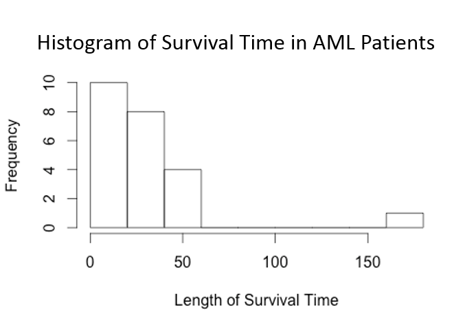
We see that the survival times are highly skewed due to the fact that there is a person who survived much longer than everyone else. In addition, there were quite a few people who survived for fewer than 10 years. This type of skewed distribution is typical when dealing with survival data and thus the normality assumption of linear regression is often violated, making it inappropriate to use.
In addition to this problem, we also see a problem known as censoring with survival data.
> leukemia[1:5,]
time status x
1 9 1 Maintained
2 13 1 Maintained
3 13 0 Maintained
4 18 1 Maintained
5 23 1 Maintained
The third observation has a status of 0. This means that the person was followed for 13 months and after that was lost to follow up. So we only know that the patient survived AT LEAST 13 months, but we have no other information available about the patient's status. This type of censoring (also known as "right censoring") makes linear regression an inappropriate way to analyze the data due to censoring bias.
Overview of Survival Analysis
One way to examine whether or not there is an association between chemotherapy maintenance and length of survival is to compare the survival distributions. This is done by comparing Kaplan-Meier plots.
> survfit(Surv(time, status)~1)
Call: survfit(formula = Surv(time, status) ~ 1)
records n.max n.start events median 0.95LCL 0.95UCL
23 23 23 18 27 18 45
This tells us that for the 23 people in the leukemia dataset, 18 people were uncensored (followed for the entire time, until occurrence of event) and among these 18 people there was a median survival time of 27 months (the median is used because of the skewed distribution of the data). The 95% confidence interval for the median survival time for the 18 uncensored individuals is (18, 45).
>summary(survfit(Surv(time, status)~1))
Call: survfit(formula = Surv(time, status) ~ 1)
time n.risk n.event survival std.err lower 95% CI upper 95% CI
5 23 2 0.9130 0.0588 0.8049 1.000
8 21 2 0.8261 0.0790 0.6848 0.996
9 19 1 0.7826 0.0860 0.6310 0.971
12 18 1 0.7391 0.0916 0.5798 0.942
13 17 1 0.6957 0.0959 0.5309 0.912
18 14 1 0.6460 0.1011 0.4753 0.878
23 13 2 0.5466 0.1073 0.3721 0.803
27 11 1 0.4969 0.1084 0.3240 0.762
30 9 1 0.4417 0.1095 0.2717 0.718
31 8 1 0.3865 0.1089 0.2225 0.671
33 7 1 0.3313 0.1064 0.1765 0.622
34 6 1 0.2761 0.1020 0.1338 0.569
43 5 1 0.2208 0.0954 0.0947 0.515
45 4 1 0.1656 0.0860 0.0598 0.458
48 2 1 0.0828 0.0727 0.0148 0.462
The following summary goes through each time point in the study in which an individual was lost to follow up or died and re-computes the total number of people still at risk (n.risk), the number of events at that time point (n.event), the proportion of individuals who survived up until that point (survival) and the standard error (std.err) and 95% confidence interval (lower 95% CI, upper 95% CI) for the proportion of individuals who survived at that point.
You can also plot the survival curves using the following commands:
> surv.aml <- survfit(Surv(time,status)~1)
> plot(surv.aml, main = "Plot of Survival Curve for AML Patients",
xlab = "Length of Survival", ylab = "Proportion of Individuals who have Survived")

This plot shows the survival curve (also known as a Kaplan-Meier plot), the proportion of individual who have survived up until that particular time as a solid black line and the 95% confidence interval (the dashed lines).
Our original question was to examine the association between chemotherapy maintenance and length of survival. To do this in the context of survival analysis we compare the survival curves of those who received chemotherapy maintenance and those who did not. First, let's examine how to compare the survival statistics and create Kaplan-Meier plots for each chemotherapy group.
> print(survfit(Surv(time,status)~x))
Call: survfit(formula = Surv(time, status) ~ x)
records n.max n.start events median 0.95LCL 0.95UCL
x=Maintained 11 11 11 7 31 18 NA
x=Nonmaintained 12 12 12 11 23 8 NA
In this output we see that there is a total of 11 people who were on maintained chemotherapy, 7 died, the median follow up was 31. The 95% confidence interval of survival time for those on maintained chemotherapy is (18, NA); NA in this case means infinity. A 95% upper confidence limit of NA/infinity is common in survival analysis due to the fact that the data is skewed.
>plot(survfit(Surv(time,status)~x), main = "Plot of Survival Curves by Chemotherapy Group", xlab = "Length of Survival",ylab="Proportion of Individuals who have Survived",col=c("blue","red"))
>legend("topright", legend=c("Maintained", "Nonmaintained"),fill=c("blue","red"),bty="n")
In order to determine if there is a statistically significant difference between the survival curves, we perform what is known as a log-rank test, which tests the following hypothesis:
- H0: There is no difference in the survival function between those who were on maintenance chemotherapy and those who weren't on maintenance chemotherapy.
- Ha: There is a difference in the survival function between those who were on maintenance chemotherapy and those who weren't on maintenance chemotherapy.
The test is performed in R as follows:
> survdiff(Surv(time,status)~x)
Call:
survdiff(formula = Surv(time, status) ~ x)
N Observed Expected (O-E)^2/E (O-E)^2/V
x=Maintained 11 7 10.69 1.27 3.4
x=Nonmaintained 12 11 7.31 1.86 3.4
Chisq= 3.4 on 1 degrees of freedom, p= 0.0653
We see that when testing the null hypothesis that there is no difference in the survival function for those who were on chemotherapy maintenance versus those who were not on chemotherapy maintenance we fail to reject the null hypothesis χ12 = 3.4 with a p-value = 0.0653.
Suppose we want to see if there is a difference in survival functions between two groups after adjusting for a potential confounder.
We will not go into much detail on this model here, but briefly, a proportional hazard model is given as follows:
We define the hazard of an event as the risk of that event, as the time frame shrinks to 0. Usually when we calculate risk ratios, we have some time in mind, either cross-sectional, or, say, risk of dying after a year for two groups. Hazard is the risk, taken as the time frame vanishes to time t = 0.
![]()
h0(t) is the "baseline hazard," which we don't worry too much about, because when we look at the ratio of hazards for two conditions, we get the following:
Hazard ratio for individual with X = x vs. X = (x+1):

This term is the hazard ratio for the event of interest for people with covariate x+1 vs. people with covariate x. If the term is >1, then those people who have a one-unit increases in their covariate compared against a reference group are at a higher "risk" (hazard) for the event.
This is just the bare-bones basics of Cox Proportional Hazards models. There is a lot more to these models, including various assumptions that need to be tested for the model validity to hold, and issues in interpretation. However, for our purposes, just seeing how to run these models is enough.
Using a new dataset in the survival package called "cancer" we want to examine the survival in 228 patients with advanced lung cancer from the North Central Cancer Treatment Group. Performance scores rate how well the patient can perform usual daily activities.
|
Variable Name |
Description |
|---|---|
|
inst |
Institution code |
|
time |
Survival time in days |
|
status |
censoring status, 1=censored, 2=dead |
|
age |
age in years |
|
sex |
1=Male, 2= Female |
|
ph.ecog |
ECOG performance score (0= good, 5=dead) |
|
ph.karno |
Karnofsky performance score (0=bad, 100=good) rated by physician |
|
pat.karno |
Karnofsky performance score as rated by patient |
|
meal.cal |
calories consumed at meals |
|
wt.loss |
Weight loss in last six months |
First, let's do some non-adjusted analysis:
|
Test the null hypothesis that there is no difference in the survival function of patients with advanced lung cancer between males and females. |

Suppose we want to determine if there is an association between length of survival and gender after adjusting for age. The log-rank test discussed previously will only compare groups, it does not take into account adjusting for other covariates/confounding variables. To adjust for other covariates we perform the Cox's proportional hazards regression using the coxph() function in R. To perform exercise 2 using Cox regression we use the following commands:
> detach(leukemia)
> attach(cancer)
> coxph(Surv(time,status)~sex)
Call:
coxph(formula = Surv(time, status) ~ sex)
coef exp(coef) se(coef) z p
sex -0.531 0.588 0.167 -3.18 0.0015
Likelihood ratio test=10.6 on 1 df, p=0.00111 n= 228, number of events= 165
We see that when using the Cox regression to perform the test, the results are very similar to the log rank test (χ12 = 10.6 with p-value = 0.00111). The Cox regression estimates the hazard ratio of dying when comparing males to females. Here, sex is significantly related to survival (p-value = 0.00111), with better survival in females in comparison to males (hazard ratio of dying = 0.588). Females have 0.588 times the hazard of dying in comparison to males.
To extend the cox regression to adjust for other covariates, we will extend this to test the following hypothesis:
- H0: There is no difference in the survival function when comparing males to females after adjusting for age.
- Ha: There is a difference in the survival function when comparing males to females after adjusting for age.
> coxph(formula = Surv(time, status) ~ sex + age)
Call:
coxph(formula = Surv(time, status) ~ sex + age)
coef exp(coef) se(coef) z p
sex -0.513 0.599 0.16746 -3.06 0.0022
age 0.017 1.017 0.00922 1.85 0.0650
Likelihood ratio test = 14.1 on 2 df, p=0.000857 n= 228, number of events= 165
When testing the null hypothesis that there is no difference in the survival function between males and females after adjusting for age we see that we reject the null hypothesis (z = -3.06, p-value = 0.0022). After adjusting for age, females have significantly better survival in comparison to males. Females have 0.599 times the hazard of dying in comparison to males, adjusting for age (HR<1).
Assignment:
- Homework 7 and Final Project report and presentation
Things we did not cover (or only touched on)
- Density Estimation (i.e., what are we really sampling from?)
- Lots more on multiple testing: Methods to control Family-Wise Error rate, False Discovery rate; Sequential Testing
- Bootstrapping: nonparametric regression, CIs, and bias estimation;
- Permutation methods for confidence intervals
- Models for correlated/structured data: Mixed-Effects Models, GEE, repeated measures analysis
- Generalized Linear Models (GLMs) and their various assumptions and interpretations (We touched only briefly on Logistic & Survival Models; there are many, many more GLMs)
- Power and sample size calculations
- R in Unix
- ggplot2 package for even better graphics http://www.statmethods.net/advgraphs/ggplot2.html
- Methods for characterizing/accounting for Missing Data
- Bayesian Statistics: Metropolis-Hastings and Gibbs sampling for estimation of posterior density functions
- Time Series data
|
For those who want to continue with R, SPH offers BS 845: Applied Statistical Modeling and Programming in R, taught by Professor Yang. |
