

Logistic Regression
Why use logistic regression?
Previously we discussed how to determine the association between two categorical variables (odds ratio, risk ratio, chi-square/Fisher test). Suppose we want to explore a situation in which the dependent variable is dichotomous (1/0, yes/no, case/control) and the independent variable is continuous.
Let's examine the Outbreak dataset in the epicalc library in R. Suppose we want to examine the association between vomiting (yes/no) as a dependent variable and age. Suppose we try to examine this association using linear regression.
E[ Vomiting ] = β0 + β1*age
If we run the linear regression model in R, what happens?
> library(epicalc)
> data(package="epicalc",Outbreak)
> attach(Outbreak)
> model.1<-lm(vomiting~age)
> summary(model.1)
> plot(model.1,which=1:4)
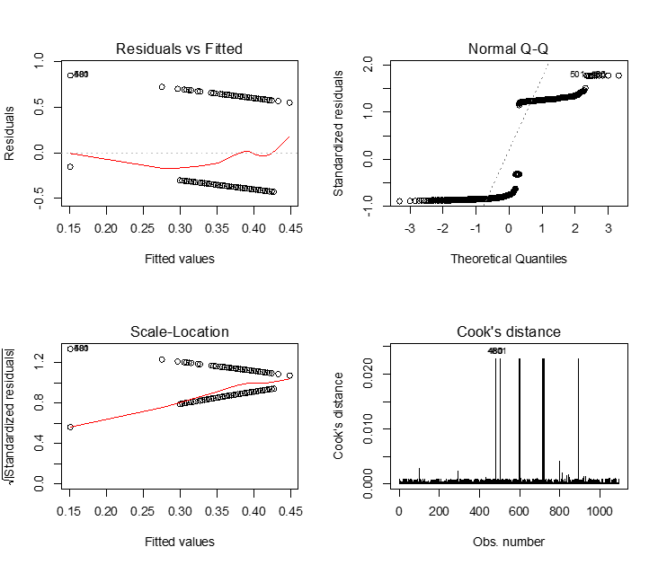
We see that just about all the assumptions of linear regression are violated in these plots. This is due to the fact that linear regression can only work well if the dependent variable is continuous. In this case the predicted values still fall between 0 and 1, which is good, but in many cases we can get an expected value of the probability of being a case that is above 1, or below 0; this is clearly erroneous.
Overview of Logistic Regression
When the assumptions of linear regression are violated, oftentimes researchers will transform the independent or dependent variables. In logistic regression the dependent variable is transformed using what is called the logit transformation:
![]()
Then the new logistic regression model becomes:
![]()
Covariates can be of any type:
- Continuous
- Categorical
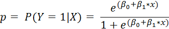
and the outcome is binary: 0/1. Since Y is either 0 or 1, expected value of Y for a set of covariates X is thought of as "the probability that event Y occurs, given the covariates X." So we have that if p is the probability of vomiting, then
![]()
In linear regression, we were able to predict the outcome Y given new data by plugging in covariates on new data into the model. Here, we can do that for odd, odds ratios, or predicted probabilities (more on this later).
In standard linear regression, the coefficients are estimated based on the "least-squares" criterion. Here, the estimates for the coefficients are performed via Maximum Likelihood Estimation.
Due to a transformed outcome, there is a concomitant change in the interpretation of the regression coefficients:
- β0 is the log odds of vomiting when age is equal to 0.
- β1 is the increase/decrease in the log odds for aGeneone-unit increase in age.
- eβ1 is the odds ratio comparing the increase/decrease in odds for those with a one-unit increase in age compared to the standard group; for example:
log(odds of vomiting for those aged 20) = β0 + β1*20
log(odds of vomiting for those aged 21) = β0 + β1*21
odds of vomiting for those aged 20 = e β0 + β1*20
odds of vomiting for those aged 21 = e β0 + β1*21
If we want to determine the odds ratio to compare the odds of vomiting for those who are 20 years old versus the odds of vomiting for those who are 21 years old we can do the following:

By laws of exponents, we can combine terms, and we get:
![]()
Thus ![]() = exp(β1) represents the odds ratio of vomiting comparing groups that differ by a one-unit change in age.
= exp(β1) represents the odds ratio of vomiting comparing groups that differ by a one-unit change in age.
If we want to get a predicted probability of the event of interest (p), given our covariates, then we can do a little algebra, and we have that
|
Generalized Linear Models |
|---|
|
There is an entire sub-field of statistical modeling called generalized linear models, where the outcome variable undergoes some transformation to enable the model to take the form of a linear combination, i.e. f (E[Y]) = β0 + β1X1+…+ βkXk. Logistic regression is just one such type of model; in this case, the function f (・) is f (E[Y]) = log[ y/(1 - y) ].
There is Poisson regression (count data), Gamma regression (outcome strictly greater than 0), Multinomial regression (multiple categorical outcomes), and many, many more. If you are interested in these topics, SPH offers · BS 853: Generalized Linear Models (logistic regression is just one class) · BS 820: Logistic Regression and Survival Analysis · BS 852: Statistical Methods in Epidemiology (covers some logistic and survival)
And in the math department there is · MA 575: Linear Models · MA 576: Generalized Linear Models |
