


Hypothesis Testing
Hypothesis testing (or the determination of statistical significance) remains the dominant approach to evaluating the role of random error, despite the many critiques of its inadequacy over the last two decades. Although it does not have as strong a grip among epidemiologists, it is generally used without exception in other fields of health research. Many epidemiologists that our goal should be estimation rather than testing. According to that view, hypothesis testing is based on a false premise: that the purpose of an observational study is to make a decision (reject or accept) rather than to contribute a certain weight of evidence to the broader research on a particular exposure-disease hypothesis. Furthermore, the idea of cut-off for an association loses all meaning if one takes seriously the caveat that measures of random error do not account for systematic error, so hypothesis testing is based on the fiction that the observed value was measured without bias or confounding, which in fact are present to a greater or lesser extent in every study.
Confidence intervals alone should be sufficient to describe the random error in our data rather than using a cut-off to determine whether or not there is an association. Whether or not one accepts hypothesis testing, it is important to understand it, and so the concept and process is described below, along with some of the common tests used for categorical data.
When groups are compared and found to differ, it is possible that the differences that were observed were just the result of random error or sampling variability. Hypothesis testing involves conducting statistical tests to estimate the probability that the observed differences were simply due to random error. Aschengrau and Seage note that hypothesis testing has three main steps:
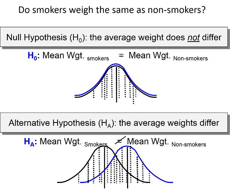
1) One specifies "null " and "alternative" hypotheses. The null hypothesis is that the groups do not differ. Other ways of stating the null hypothesis are as follows:
- The incidence rates are the same for both groups.
- The risk ratio = 1.0, or the rate ratio = 1.0, or the odds ratio = 1.0
- The risk difference = 0 or the attributable fraction =0
2) One compares the results that were expected under the null hypothesis with the actual observed results to determine whether observed data is consistent with the null hypothesis. This procedure is conducted with one of many statistics tests. The particular statistical test used will depend on the study design, the type of measurements, and whether the data is normally distributed or skewed.
3) A decision is made whether or not to reject the null hypothesis and accept the alternative hypothesis instead. If the probability that the observed differences resulted from sampling variability is very low (typically less than or equal to 5%), then one concludes that the differences were "statistically significant" and this supports the conclusion that there is an association (although one needs to consider bias and confounding before concluding that there is a valid association).
p-Values (Statistical Significance)
The end result of a statistical test is a "p-value," where "p" indicates probability of observing differences between the groups that large or larger, if the null hypothesis were true. The logic is that if the probability of seeing such a difference as the result of random error is very small (most people use p< 0.05 or 5%), then the groups probably are different. [NOTE: If the p-value is >0.05, it does not mean that you can conclude that the groups are not different; it just means that you do not have sufficient evidence to reject the null hypothesis. Unfortunately, even this distinction is usually lost in practice, and it is very common to see results reported as if there is an association if p<.05 and no association if p>.05. Only in the world of hypothesis testing is a 10-15% probability of the null hypothesis being true (or 85-90% chance of it not being true) considered evidence against an association.]
Most commonly p< 0.05 is the "critical value" or criterion for statistical significance. However, this criterion is arbitrary. A p-value of 0.04 indicates a 4% chance of seeing differences this great due to sampling variability, and a p-value of 0.06 indicates a probability of 6%. While these are not so different, one would be considered statistically significant and the other would not if you rigidly adhered to p=0.05 as the criterion for judging the significance of a result.
Video Summary: Null Hypothesis and P-Values (11:19)
Link to transcript of the video
![]()
![]()
The Chi-Square Test
The chi-square test is a commonly used statistical test when comparing frequencies, e.g., cumulative incidences. For each of the cells in the contingency table one subtracts the expected frequency from the observed frequency, squares the result, and divides by the expected number. Results for the four cells are summed, and the result is the chi-square value. One can use the chi square value to look up in a table the "p-value" or probability of seeing differences this great by chance. For any given chi-square value, the corresponding p-value depends on the number of degrees of freedom. If you have a simple 2x2 table, there is only one degree of freedom. This means that in a 2x2 contingency table, given that the margins are known, knowing the number in one cell is enough to deduce the values in the other cells.
Formula for the chi squared statistic:
One could then look up the corresponding p-value, based on the chi squared value and the degrees of freedom, in a table for the chi squared distribution. Excel spreadsheets and statistical programs have built in functions to find the corresponding p-value from the chi squared distribution.As an example, if a 2x2 contingency table (which has one degree of freedom) produced a chi squared value of 2.24, the p-value would be 0.13, meaning a 13% chance of seeing difference in frequency this larger or larger if the null hypothesis were true.
Chi squared tests can also be done with more than two rows and two columns. In general, the number of degrees of freedom is equal to the number or rows minus one times the number of columns minus one, i.e., degreed of freedom (df) = (r-1)x(c-1). You must specify the degrees of freedom when looking up the p-value.
Using Excel: Excel spreadsheets have built in functions that enable you to calculate p-values using the chi-squared test. The Excel file "Epi_Tools.XLS" has a worksheet that is devoted to the chi-squared test and illustrates how to use Excel for this purpose. Note also that this technique is used in the worksheets that calculate p-values for case-control studies and for cohort type studies.
Fisher's Exact Test
The chi-square uses a procedure that assumes a fairly large sample size. With small sample sizes the chi-square test generates falsely low p-values that exaggerate the significance of findings. Specifically, when the expected number of observations under the null hypothesis in any cell of the 2x2 table is less than 5, the chi-square test exaggerates significance. When this occurs, Fisher's Exact Test is preferred.
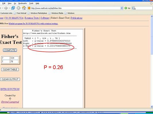
Fisher's Exact Test is based on a large iterative procedure that is unavailable in Excel. However, a very easy to use 2x2 table for Fisher's Exact Test can be accessed on the Internet at http://www.langsrud.com/fisher.htm. The screen shot below illustrates the use of the online Fisher's Exact Test to calculate the p-value for the study on incidental appendectomies and wound infections. When I used a chi-square test for these data (inappropriately), it produced a p-value =0.13. The same data produced p=0.26 when Fisher's Exact Test was used.