

Cross-Tabulation
Categorical variables may represent the development of a disease, an increase of disease severity, mortality, or any other variable that consists of two or more levels. To summarize the association between two categorical variables with R and C levels, we create cross-tabulations, or RxC tables ("Row"x"Column" or contingency tables), which summarize the observed frequencies of categorical outcomes among different groups of subjects. Here we will focus on 2 x 2 tables.
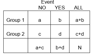
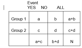
In general, 2 x 2 tables summarize the frequency of health-related (or other) events among different groups, as illustrated below in which Group 1 may represent patients who received a standard therapy, and Group 2 might be patients who received a new experimental therapy.
Example:
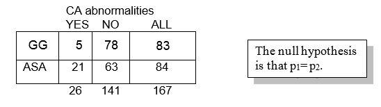
The primary outcome variable in the Kawasaki trials was development of coronary artery (CA) abnormalities, a dichotomous variable. One goal of the study was to compare the probabilities of developing CA abnormalities given treatment with Aspirin (ASA) or Gamma globulin (GG).
We might be interested in knowing whether the frequency of coronary artery abnormalities differed between these two groups, i.e., was one of these associated with fewer abnormalities. The answer to questions like this hinge on a comparison of the frequencies of these health events in the two treatment groups. Depending on the study design, one can compare either the probability of events or the odds of an event occurring.
Probability and Odds of Developing CA in Each of the Treatment Arms
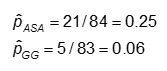
The probability is computed as the number of "yes" values in each treatment category divided by the total number in the treatment category.
The odds is #Yes / #No. Here,
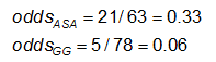
|
Always notice whether the outcome is in the rows or in the columns; it's very easy to mix these up! |

Effect Measures
When we looked at the association between one binary variable and a continuous outcome, we summarized the association in terms of difference in means. What statistics are appropriate to represent the difference between two groups with respect to the probability of a binary event? There are at least three ways of summarizing the association:
Risk Difference RD = p1 - p2
Relative Risk (Risk Ratio) RR = p1 / p2
Odds Ratio OR = odds1/ odds2 = [p1/(1-p1)] / [p2/(1-p2)]
The study design determines which of these effect measures is appropriate. In a case/control study, the relative risk cannot be assessed, and the odds ratio (OR) is the appropriate measure. However, the OR will provide a good estimate of the relative risk for rare events (i.e., if p is small, typically 0.10 or smaller).
Cross-sectional studies assess the prevalence of health measures, so the odds ratio is appropraite. With prospective cohort studies either a rate ratio or a risk ratio is appropriate, although an odds ratio can also be calculated.,
For a more detailed review of effect measures, see the online epidemiology module on "Measures of Association."
Example: Using the previous data on CA abnormalities, the effect measures for those using ASA (aspirin) versus gamma globulin (GG) are as follows:
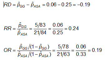

Exercise: Consider the measures of effect in the previous example. Why are the risk ratio and odds ratio so different (the RR suggests that, compared to the group treated only with ASA, the risk of coronary abnormalities is is 1/4 as high for those treated with GG; while the OR suggests the risk is 1/5 as high)?
Alternative Ways to Express the Null Hypothesis
For a 2x2 table, the null hypothesis may equivalently be written in terms of the probabilities themselves, or the risk difference, the relative risk, or the odds ratio. In each case, the null hypothesis states that there is no difference between the two groups.
H0: p1 = p2
H1: p1 ≠ p2
H0: p1 - p2 = 0 (RD=0)
H1: RD ≠ 0
H0: p1/ p2 = 1 (RR=1)
H1: RR ≠ 1
H0: OR = 1
H1: OR ≠ 1
The Chi-Square Test
The difference in frequency of the outcome between the two groups can be assessed with the chi-squared test.

In each cell of the 2x2 table, O is the observed cell frequency and E is the expected cell frequency under the assumption that the null hypothesis is true. The sum is computed over the 2x2 = 4 cells in the table. As long as the expected frequency in each cell is at least five, the computed chi-square value has a χ2 distribution with 1 degrees of freedom (df).
Reject the null hypothesis if ![]() . For α = 0.05, the critical value is 3.84.
. For α = 0.05, the critical value is 3.84.
Example:
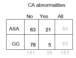
Observed frequencies
If there is no association between treatment and disease, the proportion of cases among those treated and not treated would be the same and would be equal to the proportion of cases in the entire study population.
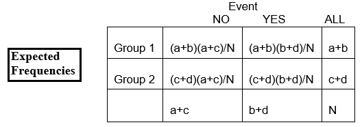
Expected frequencies:
Over all, among the 167 children, there are 26 with CA abnormalities and 141 without CA abnormalities. The proportion with CA abnormalities is 26/167, or 16%. If the null hypothesis is true, and the two treatment groups have the same probability of CA abnormalities, then we'd expect about 16% in each group to have CA abnormalities.
So, in the GG group of n=83, we'd expect 16% of 83 to have CA abnormalities. This is calculated as 0.16 x 83 = 13, and is called the expected frequency in that cell.
We can write this as
E11 = expected frequency in row 1, column 1
= expected number in group 1 who have the event (row 1, column 1)
And we calculate it as
E11 = (proportion we expect to have the event) x total number in (group) row 1
= [total number with the event (total of column 1 ) / total N] x number in (group) row 1
Using the notation in the table,
E11 = [(a+c)/N] x (a+b)
And we often rewrite this simply as
E11 = (a+b)(a+c)/N
In our example, let's calculate the expected frequency in the first cell ( E11) :
E11 = (83)(26)/167 = 12.92
We can calculate the expected frequencies in the other cells in the same way
The overall proportion without CA abnormalities is 141/167, or 84%. We expect about 84% of those in the ASA group to not have CA abnormalities, so the expected frequency in row 2, column 2, is E22 = 84% of 84, or 0.84 x 84, or approximately 71.
Using the table above, we could simply calculate it as
E22 = (c+d)(b+d)/N = (84)(141)/167 = 70.92
Exercise: How many of the children in the ASA group would you expect to have CA abnormalities if the null hypothesis is true? Try to work this out before looking at the answer below.
Note that the observed frequencies take on integer values, while the expected frequencies can take on decimal values.
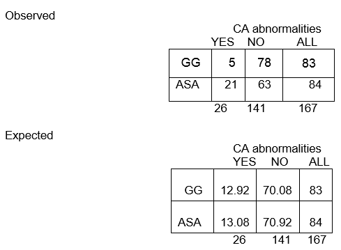
We expect nearly 13 children in the GG group to have CA abnormalities, but only 5 actually did!
Notice that once we have calculated one expected frequency, the others can be obtained easily by subtraction! The number of degrees of freedom equals the number of cells whose expected frequency needs to be calculated; in a 2 x 2 table, this is 1.
Chi-Square test statistic

where O1,1 and E1,1 are the observed and expected counts in the cell in the first row and first column. For instance, O1,1 = a and E1,1 =(a+b)(a+c)/N. If the observed cell counts are different enough from the expected, then we cannot conclude that the two probabilities are equal.

H0: The odds of CA abnormalities are the same across treatment groups (OR=1)
H1: The odds of CA abnormalities are not the same across treatment groups (OR≠1)
The significance level is 0.05.
The test statistic is calculated to be 11.43. Since our test statistic is greater than 3.84 (the chi-square critical value for 1 degree of freedom), we reject the null hypothesis and conclude that the odds of CA abnormalities are not the same in the two treatment groups.