
Measurement Error
All exposure assessments require some way of measuring exposure to a given agent, which can result in measurement error (i.e. exposure measurements determined from samples are not representative of actual exposure). Measurement error is the difference between the true exposure and a measured or observed exposure. While large inter-individual or inter-group differences can be important to detect statistically significant differences, investigators do not want such large inter-individual differences among individuals with similar exposures (i.e. between-subject variability).
Common sources of measurement error include the following:
- Faulty equipment or instruments used to estimate exposure
- Deviations from data collection protocols
- Limitations due to study participant characteristics
- Data entry and/or analysis errors
The table below uses a regression equation to demonstrate the impact measurement error can have on risk estimates in a given study. The first equation highlights what investigators want which is being able to determine the health outcome ("y") based on true exposure ("x"). However, investigators determine health outcome as a function of a measured/observed exposure ("z"). The key concern is the difference between βx and βz.
Impact on Risk Estimates
- What investigators want:
- y = α + βxx + ε
- What investigators have:
- yij= α + βzzij + εij
- α and β are coefficients to be estimated and ε is residual error.
- x = true exposure
- y = health outcome
- z = measured/observed exposure
- i = individual 'i'
- j = day 'j'
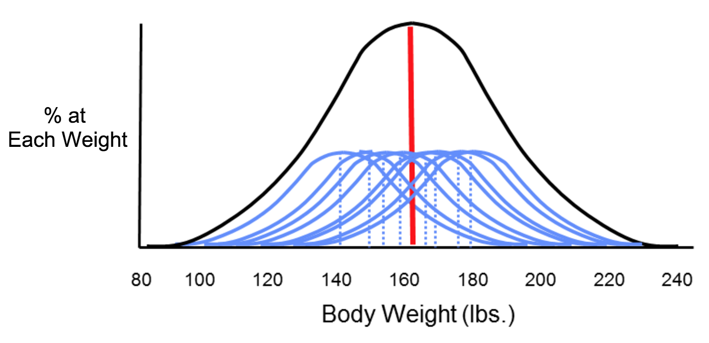
The two types of error that can result from measurements are systematic and random error, which can affect the accuracy and precision of exposure measurements. Suppose investigators wanted to monitor changes in body weight over time among the students at Boston University. In theory, they could weigh all of the students with an accurate scale, and would likely find that body weight measurements were more or less symmetrically distributed along a bell-shaped curve. Knowing all of their weights, investigators could also compute the true mean of this student population. However, it really isn't feasible to collect weight measurements for every student at BU. If investigators just want to follow trends, an alternative is to estimate the mean weight of the population by taking a sample of students each year. In order to collect these measurements, investigators use two bathroom scales. It turns out that one of them has been calibrated and is very accurate, but the other has not been calibrated, and it consistently overestimates body weight by about ten pounds.
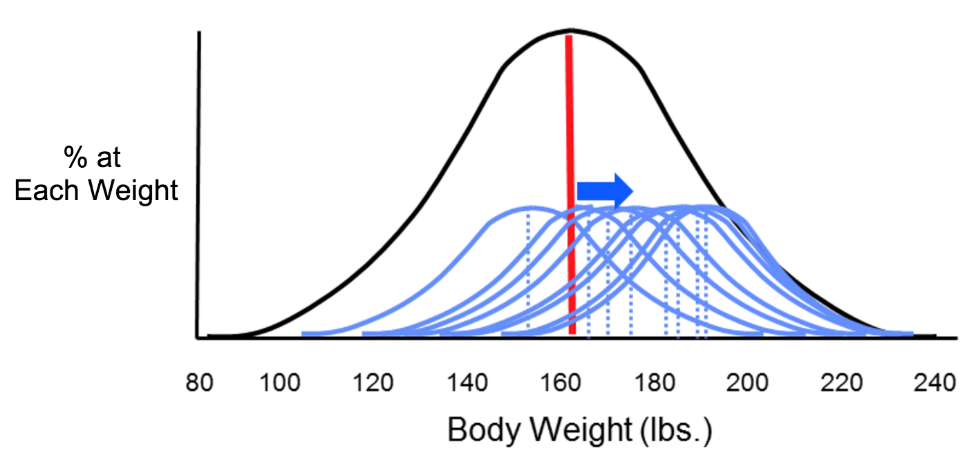
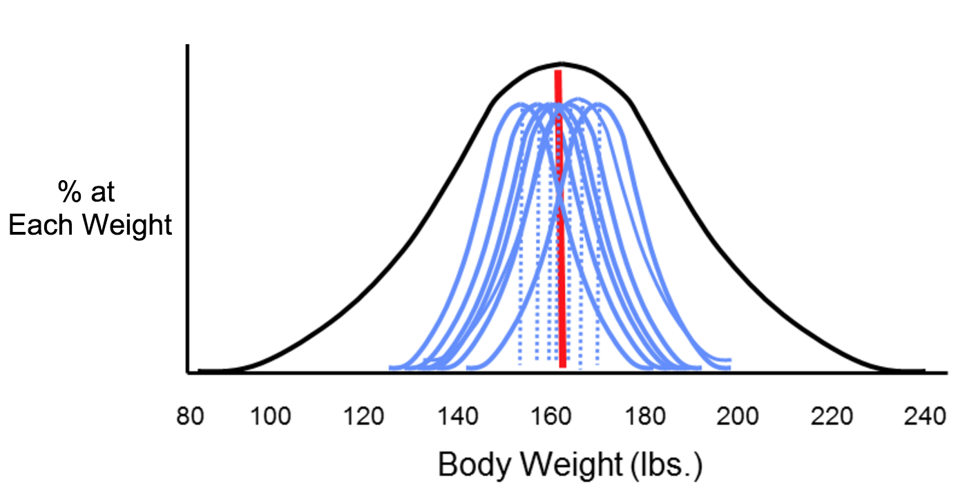
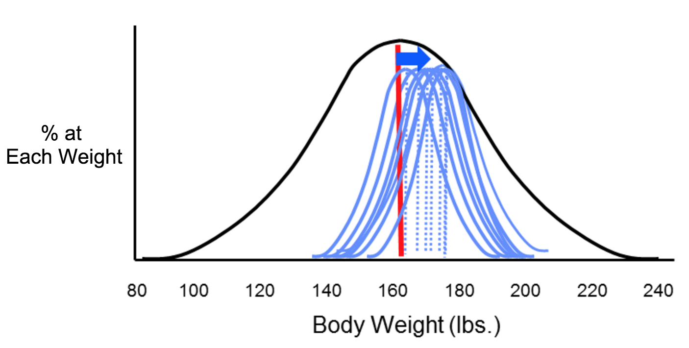
Now consider four possible scenarios as investigators try to estimate the mean body weight by taking samples. In each of the four panels (shown below), the distribution of the total population (if investigators measured it) is shown by the black bell-shaped curve, and the vertical red line indicates the true mean of the population. Review the illustration below for more information.
Small Sample Size (n = 5 students)
Larger Sample Size (n = 50 students)
Misclassification of Exposure
For environmental exposures, exposure data is often collected on an aggregate scale since individual exposure measurements can be difficult or impossible to collect, which can lead to random misclassification of exposure. Another source of random misclassification takes place as a result of the intra-individual (within-subject) variability, particularly when investigating chronic effects. For example, a study looking to assess dietary pesticide exposure may need to address how dietary intake for an individual may change seasonally, which would result in different exposure levels for the same individual.
Non-random, or differential misclassification of exposure takes place when errors in exposure are more likely to occur in one of the groups being compared. Random misclassification of exposure is when errors in exposure are equally likely to occur in all exposure groups. Random misclassification can be broken down into two categories: Berkson error model and classical error. Berkson error model refers to random misclassification that results in little to no bias in the measurement whereas classical error refers to random misclassification that tends to attenuate the risk estimates (i.e. bias towards the null).
An epidemiological study looking to examine the association between environmental tobacco smoke (ETS) and asthma exacerbation in children may define their exposed population as children living with one or more parents who smoke. What are some of the limitations regarding this classification of the exposed population?
Minimizing Exposure Error
There are measures that can be taken throughout a study (design, data collection, and analysis phase) to minimize or adjust for measurement error. For example, validation studies are studies that attempt to assess a given method of collecting exposure compared to a "gold standard." For example, a study might collect a single urine sample from study participants to analyze it for organophosphate metabolites. But the "gold standard" is to collect 24-hour urine samples. A validation study attempts to determine the level of agreement between the single urine sample and 24-hour urine samples.