


Using R to Characterize the Health of the Town
 In this exercise you will analyze a subset of the data from the Weymouth Health Survey using R in order to characterize and describe the some of the pertinent risk factors and health outcomes in Weymouth and to begin to explore some of the potentially important associations between modifiable behaviors and health outcomes. This is an exercise designed to give you more practice using the R statistical package. You should complete this exercise on your own after the first Lab exercise which is an "Introduction to Using R".
The JSI household survey was very extensive in that it included many questions, and the household member who responded was asked to provide responses for each of the adults (18 years of age and above) in the household. The data set below is a modified version of the JSI data set that includes only data from the primary respondents, and it has been pared down to selected variables. The data has also been cleaned and reformatted for some variables for this exercise. Here is a link to the modified version of the data collected from the household survey:
The variables in this data set are described in the file below, which contains the abbreviated names of the variables that are used as column headers in the data set, and there is also a brief explanation of the question that was asked and the possible responses.
Link to the variable key for Weymouth_-Part.CSV
After the first Lab exercise on using R, review the course module entitled R Basics for PH717 , load the Weymouth_Adult_Part.CSV data set into R and complete the exercises below. Note that we are providing both the R code and the output that you should expect to see, since the purpose of this exercise is to give you addtional practice using R and to familiarize you with real data from the Weymouth Health Survey.
#### Part 1 ####
# The first command below creates a data frame object called 'wey'.
# The "na.omit" portion asks R to omit missing data points (which are NA or not available)
> wey<-na.omit(Weymouth_Adult_Part)
#Next, attach the data set
> attach(wey)
# Create a derived variable for the respondents age in 2002 based on the reported birth year.
> age=(2002-birth_yr)
# Compute body mass index (BMI) as shown in the line below
> bmi=weight/hgt_inch^2*703
# Compute the mean and standard deviation of BMI
> mean(bmi)
[1] 26.93121
> sd(bmi)
[1] 5.393322
# Create a contingency table for history of myocardial infarction (hx_mi) and history of diabetes mellitus (hx_dm)
> table(hx_mi,hx_dm)
hx_dm
hx_mi 0 1
0 1815 138
1 70 36
# Among those with or without diabetes, what proportion had had an MI?
> prop.table(table(hx_mi,hx_dm))
hx_dm
hx_mi 0 1
0 0.88149587 0.06702283
1 0.03399709 0.01748422
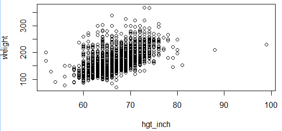
#Compute the correlation coefficient for height and weight
> cor(hgt_inch,weight)
[1] 0.5653241
# Make a scatter plot of height and weight
> plot(hgt_inch,weight)
# Compute the correlation coefficient for age and BMI
> cor(age,bmi)
[1] 0.04977146
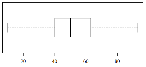
# Create a boxplot for age with horizontal orientation
> boxplot(age,horizontal = T)
#Create a histogram of age and a histogram of BMI
> hist(age)
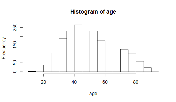
> hist(bmi)
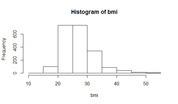
You can modify the appearance of the histogram by adding additional arguments to the code, such as the following:
hist(bmi, main="BMI Distribution in Weymouth Adults", xlab="BMI", border="blue", col="green", xlim=c(10,50), las=1, breaks=8)
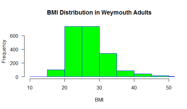
Are age and BMI reasonably normally distributed?
Based on this histogram, what would you conclude about the distribution of BMIs in Wey mouthy adults?
# Compute the mean and standard deviation for age
> mean(age)
[1] 51.68431
> sd(age)
[1] 15.70907