Weymouth
Building a Healthy Weymouth
A Brief History of Weymouth, MA
 The Town of Weymouth occupies 21.6 square miles about 12 miles south of Boston on the South Shore. It is the second oldest settlement in the Commonwealth of Massachusetts, dating from 1622. Thomas Weston, a London merchant, had done helped finance the Pilgrims and pay for the Mayflower, because he believed that there was the potential for a lucrative business based on trade with the colonies. Since the Pilgrims were motivated more by religious freedom than investment opportunities, Weston wanted to establish a separate colony that would serve as a trading post from which lumber, furs, salted fish could be shipped to England. Accordingly, he sent 60 men to what is now North Weymouth and named it "Wessaguscus" or "Wessagusset". These sixty men were apparently unprepared for the rigors that faced them, especially during the harsh winters. Food stores dwindled rapidly, and the men were forced to eke out an existence by foraging for shellfish, nuts, and berries. With starvation threatening, they appealed to the Plymouth colony for food, but they too had scarce supplies. The Wessagusset men first resorted to trading clothing and other wares to the local Indians in exchange for food. When their wares ran out, they resorted to working for the Indians in exchange for food or simply stealing food from them.
By 1623 the Indians were becoming increasingly irritated with the new settlers, and it was rumored that they intended to wipe out the Wessagusset settlement and then attack the Plymouth settlers. One of the Wessagusset men got word to Miles Standish in Plymouth, and Standish took a band of men to Wessagusset and made a preemptive strike, killing the Indian chief Pecksuot and and several of his men. Many of the Wessagusset men subsequently moved to Plymouth and others to Maine; two of the men who remained a Wessagusset were killed by the Indians in retaliation for the attack by Miles Standish.
Six months later Robert Gorges, a captain in the British navy, obtained a grant and brought approximately 120 men and women from Weymouth, England to the Wessagusset colony. Gorges and some of the settlers returned to England in 1624, but others remained in the colony that they renamed "Weymouth. One of the ministers in the Gorges expedition was the Reverend William Blaxton (also spelled Blackstone), who shortly thereafter became the first settler in what is now Boston. The Weymouth colony slowly grew, and by 1633 it was described as follows:
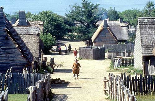
"... yet but a small village, yet it is very pleasant and healthful, very good ground and is well timbered, and hath good store of hay ground. It hath a spacious harbor for shipping before the town, the salt water being navigable for boats and pinnaces two leagues. Here the inhabitants have good store of fish of all sorts, and swine, having acorns and clams at the time of the year. Here is likewise an alewife river."
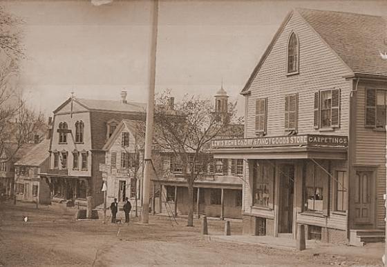
The early settlement must have looked much like the one depicted below.
.

A Favorable Location for Early Industries
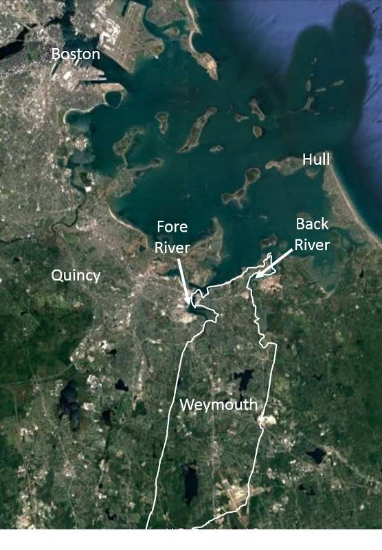
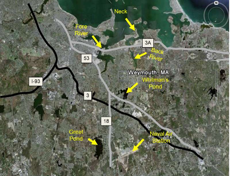
The map above on the right shows the outline of Weymouth bordered on the north by Quincy Bay, which is part of Boston Harbor. In addition to shipping access, Weymouth also enjoyed a fair amount of protection from Hull peninsula, and Weymouth was also bounded by the Fore River to the west and the Back River to the east, providing not only additional havens for ships, but also the opportunity to erect mills and a shipbuilding industry.
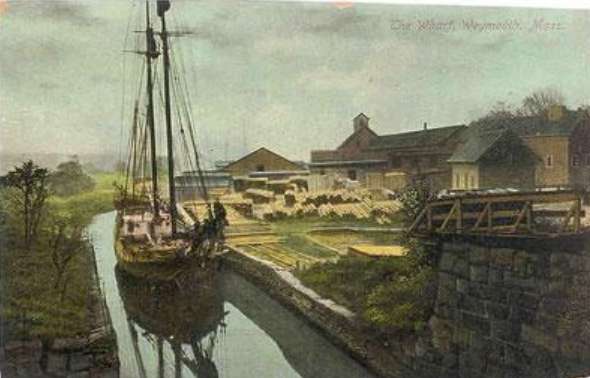
The image below shows a schooner at Rhines lumber yard in Weymouth Landing which is upriver from the mouth of the Fore River.
In the 1630s Wessagusset became recognized as part of the Massachusetts Bay Colony. In 1635 21 new families arrived from Weymouth, England, and the town was renamed Weymouth. The settlers lived primarily on fishing and farming, and they also harvested lumber from the forests and salt and thatch from its salt marshes.
Eventually, other communities began to spring up, and, like many of them, Weymouth was governed by a town meeting which met at least twice a year (March and November). The town meeting established local laws and regulations and levied fines and taxes. For example, laws were established to protect the salt marshes, which were an important source of salt and thatch. Other laws were enacted to manage the harvesting of pine and cedar that were important resources for construction and export.
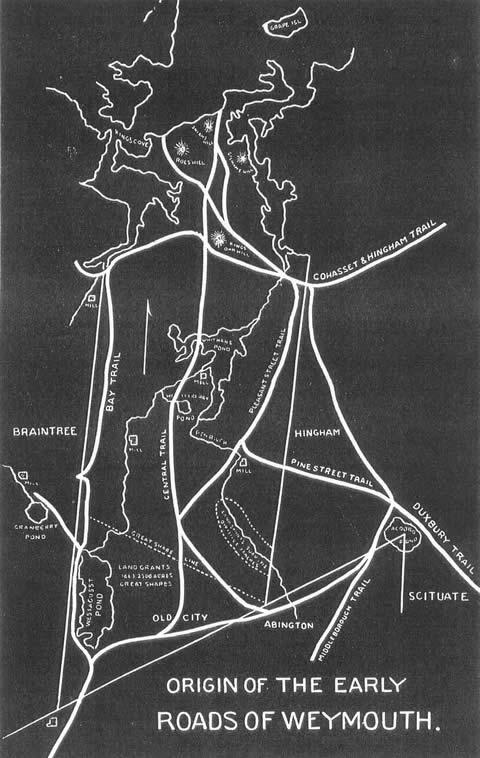
As the town grew, the simple network of paths originally used by the Indians gave rise to roads that expanded Weymouth southward from the bay to Whitman's Pond and also connected it to other communities. Ferries began to connect Weymouth to Boston and other communities, and town meetings took up the business of planning, building, and maintaining roads and bridges.
Indian Wars
From 1636-37 the Pequod War took place in southern New England, which pitted the Pequod tribe against an alliance of other tribes and the English settlers. The Pequods lost the war, and a period of relative peace followed, but the growing demands of the English settlers for more and more land continued to cause friction with the Native Americans, including the local Wampanoag Indians. Chief Massasoit had worked to help the English and maintain a good relationship. His son Metacom, also know as "King Philip", succeeded him, and in 1671 he was forced to sign a humiliating peace treaty that required his tribe to surrender their guns. In 1675 and Indian who was an informer for the English settlers was murdered, and officials in the Plymouth colony tried three Wampanoags for the murder and executed them by hanging. Metacom was incensed and ordered an attack on Swansee and other settlements in retaliation, thus triggering "King Philip's War."

Source: http://www.executedtoday.com/tag/king-philips-war/
The conflict was widespread, and some of the fighting occurred in Weymouth where houses and barns were burned by the Indians on several occasions. Eventually, the Indians were defeated. King Philip was assassinated by a Native American working for the English, and his head was impaled on a pike in Plymouth. The war was costly to the settlers, but it devastated the Wampanoags, and the expansion of settlements proceeded without further opposition.
New Industries and Trades
As the town grew, manufacturing, trades, and retail businesses began to spring up. Soon there were merchants, manufacturers, and tradesmen. At first, cobblers were itinerant tradesman who went from farm to farm and fashioned shoes for all members of the family from the cowhides provided by the farmer. But by 1700 many farmers had become adept at making their own boots, and they began to create small shops on their farms called "ten footers" for boot making.

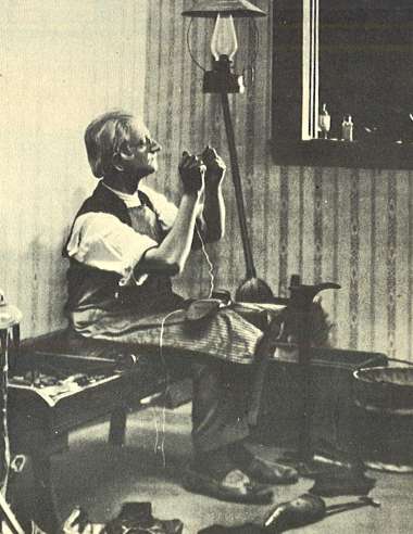
Source: http://www.weymouth.ma.us/sites/weymouthma/files/file/file/shoe_industry.pdf
Initially, boot making was simply a way to "do it yourself" to save money, but it became an additional source of income. As demand for boots and shoes increased the shoemakers began to specialize and collaborate, passing a pair of boots or shoes shoes from one craftsman to the next until it was finished.
The town continued to thrive and expand supported by an array of manufacturing and businesses. The population grew and more homes were constructed. By 1720 there were about 100 families living in small neighborhoods in what is now South Weymouth.
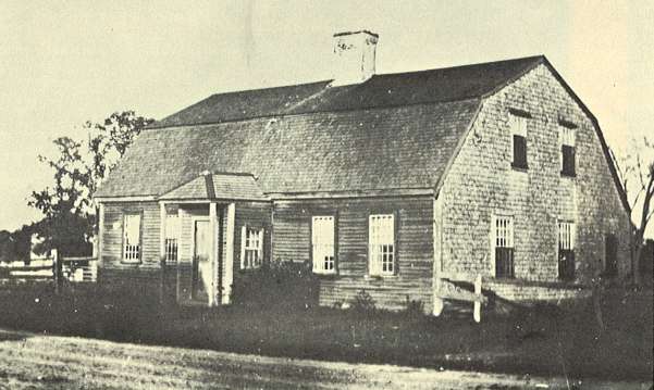
The Warren Thayer house built in 1728 on Pond Street
Source: http://www.weymouth.ma.us/sites/weymouthma/files/file/file/homes.pdf
Weymouth also hosted a number of taverns such as the Arnold Tavern (below) which was built in 1740
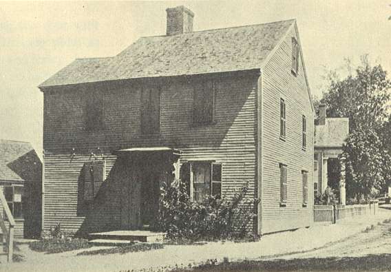
Arnold's Tavern in Weymouth Landing was built in 1740
Source: http://www.weymouth.ma.us/sites/weymouthma/files/file/file/toll_houses.pdf
The first shoemaking factory in Weymouth was founded by James Tirrell in 1808. The factory was located on Front St. near Reed's Cemetery. More factories opened. Initially, they were small to medium-sized factories, but over time they became larger and larger.
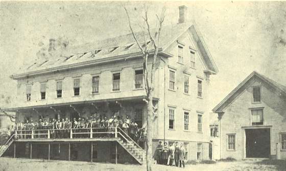
Tirrell Shoe Factory
Sources: http://www.weymouth.ma.us/sites/weymouthma/files/file/file/shoe_industry.pdf
A deposit of bog iron had been found in Great Pond in 1770, and began to be used to manufacture nails. Bog iron was also discovered in Whitman's Pond, and in 1837 the Weymouth Iron Works was founded there.
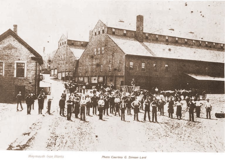
Weymouth Iron Works
Source: http://www.weymouth.ma.us/sites/weymouthma/files/file/file/iron_industry.pdf
Health
Weymouth's First Physician
Dr. James Torrey was born in Connecticut in 1756. His first occupation was as a tanner of hides, but he then apprenticed in medicine and practiced in Lebanon, CT and then on Nantucket. He served six weeks as surgeon's mate in the Revolutionary War and was later commissioned as surgeon of the Second Regiment, First Brigade, First Division, Massachusetts Militia. In 1783 he opened a practice in South Weymouth at the corner of Pleasant St. and Union Street. For more than thirty years he was the only physician in South Weymouth until he died at the age of 61.
US Public Health Starts in Massachusetts
In 1799, The Boston Board of Health was established to combat any potential cholera outbreaks. Paul Revere was Boston's first health commissioner
In 1842 - Lemuel Shattuck, a Massachusetts legislator, established the first US system for recording births, deaths and marriages. Largely through his efforts Massachusetts legislation became the model for all the other states in the Union. Among Shattuck's many contributions were his proposal for a standard nomenclature for disease; establishment of a system for recording mortality data by age, sex, occupation, socioeconomic level, and location; the application of data to programs in immunization, school health, smoking, and alcohol abuse.
In 1849 the Massachusetts legislature appointed a Sanitary Commission 'to prepare and report to the next General Court a plan for a sanitary survey of the State', with Shattuck as Chief Commissioner and author of its report. The report (1850) was enthusiastically received by the New England Journal of Medicine, but the 50 recommendations in the report were otherwise ignored. Twenty years later the Secretary of the Board of Health of Massachusetts based his plans for public health on Shattuck's recommendations.
In 1844 the Old Colony Railroad was chartered to build a railroad from Boston to Plymouth.
In 1864 the Boston City Hospital opened.
Continued Development
With the growth of local industry and commerce and the development of railroads in the mid-1800's, the Town prospered, and by 1870 the population had grown to over 6,000. Weymouth even became somewhat of a destination for residents in the Boston area. The print below shows Lovell's Grove in North Weymouth in 1875 viewed from Quincy Point to the west. There is a small park in the center, and pleasure boaters can be seen in the Fore River. The steamship Massasoit can be seen docked at Downer's Landing on the left after bringing sightseers from Boston, and vehicles and strollers can be seen on the Old Colony Road bridge.
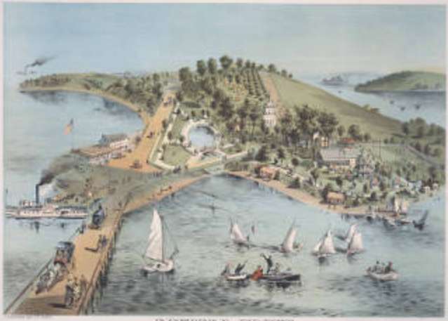
Lovell's Grove, Weymouth, MA
Source: http://cdm.bostonathenaeum.org/cdm/ref/collection/p13110coll5/id/955
The Bradley Fertilizer Company (pictured below) was founded on the point of land adjacent to the Back River on Weymouth Neck in 1874 and remained in operation until 1982 when it was purchased by ConocoPhillips. They, in turn, sold the land to the Weymouthport Peninsula Corporation in 1967, and the manufacturing buildings were demolished for redevelopment. Condominiums were built in this area in the 1970s and 1980s. In the late 1990s environmental sampling at the site revealed elevated levels of arsenic and lead at the site. ConocoPhillips agreed to pay for clean up and remediation of the site.

Source: http://cdm.bostonathenaeum.org/cdm/ref/collection/p13110coll5/id/5
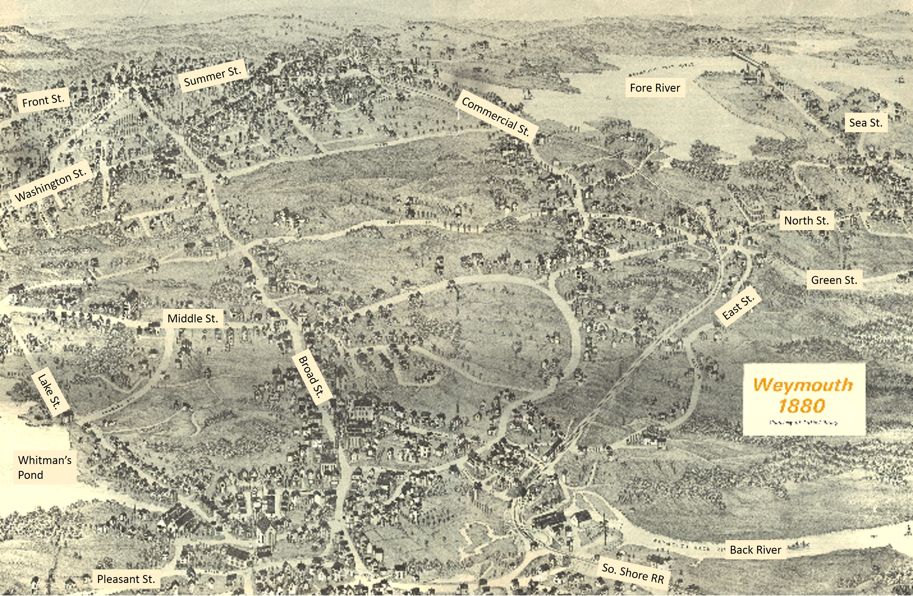
Weymouth in 1880
Adapted from http://www.weymouth.ma.us/sites/weymouthma/files/file/file/illustrated_maps_1.pdf
Link to a large PDF of this map and a map of the original footpaths in Weymouth
From http://www.weymouth.ma.us/history
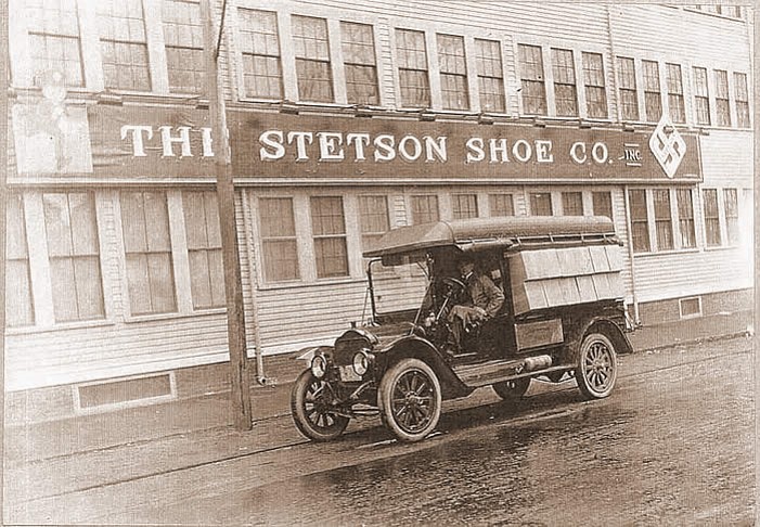
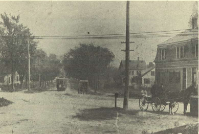
"When Weymouth's iron industry declined in the face of competition from Pennsylvania steel mills, the shoe industry rose to the economic forefront. Shoe manufacturing employed about 75 percent of community residents, and along with some other manufacturing ventures, it supported Weymouth's economy through World War II. Immigration helped supply the workforce for the new businesses, and arriving cultures helped populate the town (along with the rest of the Great Boston region). Although Weymouth was linked by streetcars and railroads to surrounding communities, most of the local retail and service businesses were in close proximity to one another and within walking distance of many homes. This was an era when local corner stores thrived on foot traffic."
In 1882 The Stetson Shoe Co. was the last of the shoe factories to open in Weymouth. It remained in operation until the 1960s.
Weymouth's Four Village Centers
One thing that distinguished Weymouth from most other New England towns is that it does not have a clearly identifiable central commercial area or "downtown" area. Instead, four smaller village centers evolved, probably emerging from what began as clusters of houses and small shops at a particular crossroads. The four villages remain distinct and identifiable today, although their importance and commercial stability has been progressively undermined by the development of large shopping malls and entertainment complexes elsewhere on the South Shore that can be reached by car (e.g., South Shore Plaza in Braintree, The Derby Street "Shoppes" in Hingham", and the Hingham Shipyard, which now provides a movie theater complex and an array of restaurants and shops.
Bicknell Square in North Weymouth
Bicknell Square is now the focal ;point for commerce in North Weymouth along what is now Bridge St. or Route 3A. One can stat at the intersection of Sea St and Bridge St. (Route 3A). You can visit the area via Google Earth by typing the address "413 MA-3A" into the Search box at the upper left corner of Google Earth.
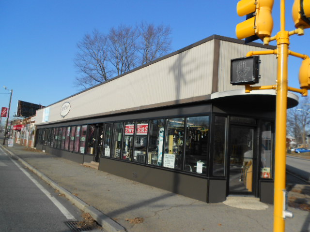
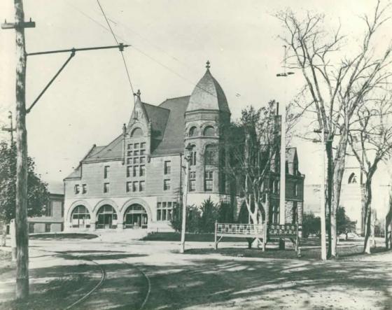
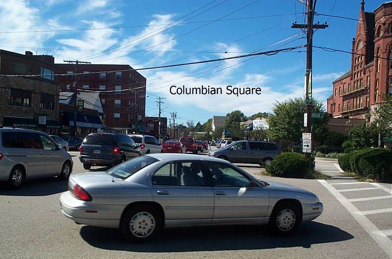
Columbian Square in South Weymouth
You can visit Columbian Square via Google Earth by typing the address "56 Columbian St., Weymouth, MA" into the Search box at the upper left corner of Google Earth. The photo below on the left shows the Fogg Opera House around 1900; in the photo on the right it is the brick building at the far right.
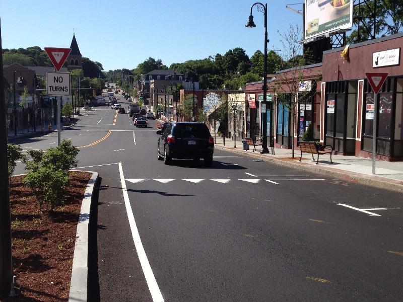
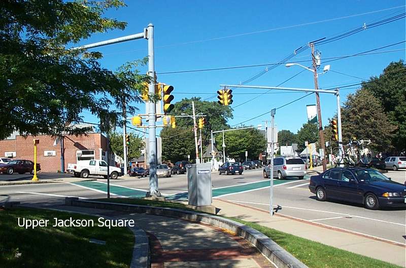
Lower Jackson Square (Commercial Square) in East Weymouth
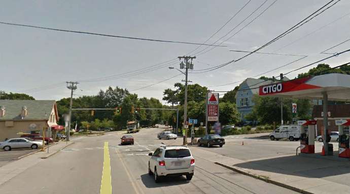
You can visit Lower Jackson Square via Google Earth by typing the address "961 Broad St., Weymouth, MA" into the Search box at the upper left corner of Google Earth. Niko's Restaurant with the red awning is at the site of Burrell's Store (there is a green street sign on the corner that says "Burrell's Corner". Across the street one can still see the original Washington St. School built in 1887 (the large blue building on the corner of High St. and School St. In the photos below the peaked building on the left was Burrell's store (now Niko's restaurant), and the Washington St. School building is on the right side of the image (blue building in the distance just left of the Citgo sign in the image on the right).
.jpg)
Weymouth Landing
To visit Weymouth Landing with Google Earth type "49 Commercial St, Weymouth, MA" into the search box, and then drag the person icon onto the street to see the street view and the shops as they are today.
Post War Evolution of the Town
After World War II, a number of other factors contributed to a substantial transformation of the town. Rising incomes led to the explosion in automobile ownership, and there was aggressive development of highways, including the bisection of the town by route 3 in 1956.
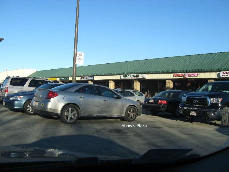
Commuter rail service was discontinued. The general expansion of the population was further fueled by migration out of the cities into the suburbs. With the advent of the route 3 expressway and other new road construction, residents began commuting to other locations for their jobs. The shoe factories closed and the local economy became largely based on smaller service, retail and some wholesale operations to support the new neighborhoods. Local retail was replaced by large malls at South Shore Plaza in Braintree and Hanover Mall in addition to a number of smaller "strip malls" in Weymouth and adjacent towns. The largest employer in town is now South Shore Hospital, and the old Stetson Shoe Factory on Route 18 now houses an array of medical offices. Most residents now commute to Boston or other cities. Ultimately, these shifting trends resulted in heavy reliance on automobiles, with overcrowding of local roads and highways, steady erosion of small, local businesses, and a gradual loss of "walkability and access to local retail within the community.

The rise of the automobile and the proliferation of highways and roads had brought convenience and many benefits to Weymouth, but it also divided the town into many separate islands that were only accessible by automobile.
Optional Video Overview of Weymouth's History
This is an optional 30 minute review of the history of Weymouth produced by the educational cable station in Weymouth (WETC ).
Then and Now
Let's explore Weymouth as it is today and compare and contrast it with Weymouth as it existed in 1880.
Install Google Earth on your computer if you don't already have it. If you don't yet have it, go to https://www.google.com/earth/ and install the free version. After Google Earth is installed and you have opened it, you will see a search box at the upper left corner of your screen. Enter "75 Middle St., Weymouth, MA," which is the street address for the current town hall. Hit the enter key. This will zoom down the Weymouth. At the lower left corner of your Google Earth window, there is a sub window for "Layers" with a series of options that you can turn on or off. Click on the boxes for
- Borders and labels
- Roads
- 3D Buildings
Navigation:
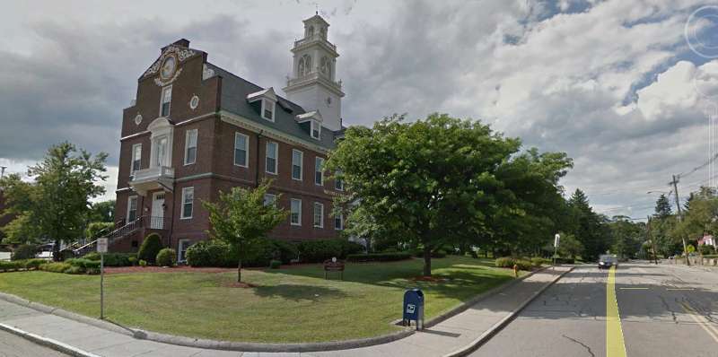
You can navigate using the controls on the left side of the Google Earth window. The top control rotates the direction of view; the next control is for tilt, and the third one is for zooming in and out. Note the small person icon that allows you to enter "street level view" for a closer look by clicking on the person icon and dragging it to the desired location on the map. The first image below is of the Weymouth Town Hall, and the next is the Town Hall from the street level view. Note that you can navigate from either view.
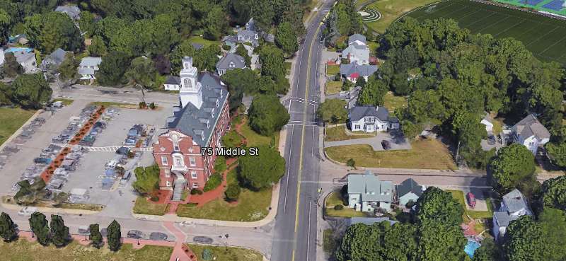
The street level view of the Weymouth Town Hall as seen from Google Earth (below):
Now take yourself on a tour of Weymouth to get a sense of its layout and resources. Start your exploration while zoomed out to get an overview. Then explore in greater detail will zoomed in, wit h or without the street level view.

Reflect on the picture of Weymouth that emerges from the historical description and the map above showing the state of Weymouth in 1880. What are the keys differences? Think both broadly and deeply. Consider any differences that might have an impact on the health of the population, including population density, roads, transportation, places of business, etc. Compose your thoughts in no more than 300 words, and post them in the Discussion Forum for this assignment on Blackboard.
The Weymouth Health Survey
From 2002-2003 Weymouth hired John Snow Inc. (JSI) to conduct surveys to assess the health status of the town in order to identify unmet health needs and modifiable risk factor that might provide opportunities to improve health. An extensive health questionnaire was mailed to 5,000 households in Weymouth. In addition, a separate survey focusing on behaviors known to contribute to leading causes of death and disability among youth and young adults was conducted among all 3,400 Weymouth public school students in grades six through twelve.
Here are links to the two surveys:
- Weymouth Household Survey Questionnaire
- Weymouth School Survey Questionnaire
You need not read the entire surveys, but take a look at them to get a feel for the format of a professionally constructed questionnaire and the level of detail.
The data was analyzed and reported to the town by JSI and highlights of their report are summarized below.
Highlights from the Household Survey
- Weymouth has higher rates of high blood pressure than the comparison samples. (33.3 %, Weymouth ; 23.6 % MA; 25.8 % US)
- Adults in low income households have particularly higher rates of high blood pressure than comparison samples (51.4% Weymouth; 33.0% MA; 34.3% US).
- Weymouth has higher rates of high cholesterol than the comparison samples. (39.5 % Weymouth, 29.7 % MA; 30.9 % US).
- Subgroups in Weymouth have notably higher rates of high cholesterol than the same subgroups in the comparison samples; men (43.6 %), those over 65
- (52.6 %) and those from lower income households (51.3 %).
- Weymouth diabetes rates of 8.7 % are significantly higher than Massachusetts (5.6 %) and slightly higher than the US (6.8 %).
- Subgroups in Weymouth have notably higher rates of diabetes than the same subgroups in the comparison samples; men (11.7 %), those from lower income households (17.0 %) and those over 65 (16.8 %).
- Weymouth residents with diabetes were less likely to have had a diabetes-related medical visit within the past 12 months than residents in the comparison samples (87.5 %, Weymouth, 91.5 %, MA and 90.2 %, US).
- Weymouth residents with diabetes are less likely than those in Massachusetts comparison sample to take oral medication (59.1 % vs. 67.0 %); to have taken a diabetes management class (43.8 % vs. 57.7 %), or to use insulin (23.5 % vs. 29.1 %).
- More Weymouth residents report shortness of breath than those nationally (38.8 % vs. 31.5 %).
- More Weymouth residents report being overweight than the comparison sample (63.3 %, Weymouth; vs. 53.3 % US).
- Objective Body Mass Index show that more Weymouth residents are overweight than in the comparison samples (31.2 % obese, Weymouth; 16.6 % obese, MA; 21.6 % obese, US).
- Among Weymouth adults who drink, 14.9 % are considered to be "at risk" for developing drinking problems. This is considerably higher compared to the state and national samples (9.8 % and 8.7 %, respectively).
- Male drinkers were more likely to be "at risk" than in the comparison samples (Weymouth, 19.2 %; MA, 10.6 %; US, 9.9 %).
- Elderly drinkers (adults 65 years or older) in Weymouth more "at risk" compared to state and national samples. (Weymouth, 23.0 %; MA, 12.9 %; US, 12. 5 %).
JSI Summary
Link to JSI Summary of the Weymouth Health Survey
Just read pages 1-4 of the Executive Summary in the JSI report at the link above.
The results of the survey raised concerns among the residents, as reported in the article below from The Boston Globe.
Other Surveys Used to Assess Youth Behaviors
Massachusetts Youth Health Survey (MYHS)
From www.mass.gov/eohhs/gov/departments/dph/programs/admin/dmoa/health-survey/myhs/
"The Massachusetts Youth Health Survey (MYHS) is the Massachusetts Department of Public Health's (MDPH) surveillance project to assess the health of youth and young adults in grades 6-12. It is conducted by the MDPH Health Survey Program in collaboration with the Massachusetts Department of Elementary and Secondary Education (ESE) in randomly selected public middle and high schools in every odd-numbered year. The anonymous survey contains health status questions in addition to questions about risk behaviors and protective factors.
Early in 2006, ESE and DPH began discussions with University of Massachusetts Center for Survey Research (CSR) and the CDC to coordinate the YHS and the ESE's Massachusetts Youth Risk Behavior Survey (YRBS) efforts in order to decrease the burden placed on the schools. The two agencies developed revised versions of the YHS and YRBS surveys. Since 2007, CSR has administered both the YHS and YRBS, and joint reports have been released on the findings.
Youth Risk Behavior Surveillance System (YRBSS)
Link to YRBSS web site
The Youth Risk Behavior Surveillance System (YRBSS) is a national school-based survey that monitors health-risk behaviors contributing to the leading causes of death and disability among youth and adults
- Behaviors that contribute to unintentional injuries and violence
- Sexual behaviors related to unintended pregnancy and sexually transmitted diseases, including HIV infection
- Alcohol and other drug use
- Tobacco use
- Unhealthy dietary behaviors
- Inadequate physical activity
YRBSS also measures the prevalence of obesity and asthma and other priority health-related behaviors plus sexual identity and sex of sexual contacts.
Using R to Characterize the Health of the Town
In this exercise you will analyze a subset of the data from the Weymouth Health Survey using R in order to characterize and describe the some of the pertinent risk factors and health outcomes in Weymouth and to begin to explore some of the potentially important associations between modifiable behaviors and health outcomes. This is an exercise designed to give you more practice using the R statistical package. You should complete this exercise on your own after the first Lab exercise which is an "Introduction to Using R".
The JSI household survey was very extensive in that it included many questions, and the household member who responded was asked to provide responses for each of the adults (18 years of age and above) in the household. The data set below is a modified version of the JSI data set that includes only data from the primary respondents, and it has been pared down to selected variables. The data has also been cleaned and reformatted for some variables for this exercise. Here is a link to the modified version of the data collected from the household survey:
Weymouth_Adult-Part.csv
The variables in this data set are described in the file below, which contains the abbreviated names of the variables that are used as column headers in the data set, and there is also a brief explanation of the question that was asked and the possible responses.
Link to the variable key for Weymouth_-Part.CSV
After the first Lab exercise on using R, review the course module entitled R Basics for PH717 , load the Weymouth_Adult_Part.CSV data set into R and complete the exercises below. Note that we are providing both the R code and the output that you should expect to see, since the purpose of this exercise is to give you addtional practice using R and to familiarize you with real data from the Weymouth Health Survey.
#### Part 1 ####
# The first command below creates a data frame object called 'wey'.
# The "na.omit" portion asks R to omit missing data points (which are NA or not available)
> wey<-na.omit(Weymouth_Adult_Part)
#Next, attach the data set
> attach(wey)
# Create a derived variable for the respondents age in 2002 based on the reported birth year.
> age=(2002-birth_yr)
# Compute body mass index (BMI) as shown in the line below
> bmi=weight/hgt_inch^2*703
# Compute the mean and standard deviation of BMI
> mean(bmi)
[1] 26.93121
> sd(bmi)
[1] 5.393322
# Create a contingency table for history of myocardial infarction (hx_mi) and history of diabetes mellitus (hx_dm)
> table(hx_mi,hx_dm)
hx_dm
hx_mi 0 1
0 1815 138
1 70 36
# Among those with or without diabetes, what proportion had had an MI?
> prop.table(table(hx_mi,hx_dm))
hx_dm
hx_mi 0 1
0 0.88149587 0.06702283
1 0.03399709 0.01748422
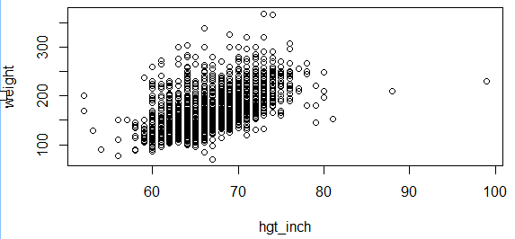
#Compute the correlation coefficient for height and weight
> cor(hgt_inch,weight)
[1] 0.5653241
# Make a scatter plot of height and weight
> plot(hgt_inch,weight)
# Compute the correlation coefficient for age and BMI
> cor(age,bmi)
[1] 0.04977146
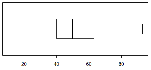
# Create a boxplot for age with horizontal orientation
> boxplot(age,horizontal = T)
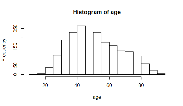
#Create a histogram of age and a histogram of BMI
> hist(age)
> hist(bmi)
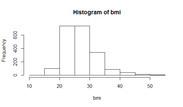
You can modify the appearance of the histogram by adding additional arguments to the code, such as the following:
hist(bmi, main="BMI Distribution in Weymouth Adults", xlab="BMI", border="blue", col="green", xlim=c(10,50), las=1, breaks=8)
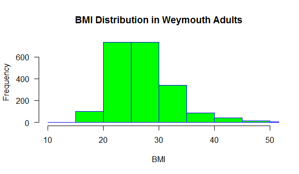
Are age and BMI reasonably normally distributed?
Based on this histogram, what would you conclude about the distribution of BMIs in Wey mouthy adults?
# Compute the mean and standard deviation for age
> mean(age)
[1] 51.68431
> sd(age)
[1] 15.70907
What Is the Next Step?
Based on your summary of the problems in Weymouth, how should they proceed?
Who are the stakeholders?
How might these concerns be dealth with in the town of Weymouth?
What interventions might improve the health of the adults in Weymouth?
What interventions might improve the health of children?
Who should take the lead?
What are the next steps?
Possible stakeholders and their reactions:
- State and local physicians feel that this is a medical problem that is best dealt with one-on-one between patients and their providers.
- A local business owner, specializing in health and nutrition, says that "People need to be educated about the benefits of healthy eating and exercise, and we need to motivate people to adopt healthy habits."
- The superintendent of schools says, "We need more resources for health education and physical education in schools."
- Local restaurant owners say, "I run a business. I provide what people want and what they will buy."
- Health teachers in the school system say, "The students don't listen. I think I know what is healthy, and we try to tell them, but they don't listen."
- A parent says, "I'm at a loss. Everyone in my family is constantly busy and on the run. It's tough to plan meals for all of us. And besides the recommendations for healthy eating keep changing."
- The woman who chairs the local board of health wants to propose a town ordinance that bans fast food restaurants in Weymouth.
- A selectman wants to propose a town tax on fast foods and on sugary soft drinks.
Is Overweight/Obesity a Health Problem?
The increased prevalence of obesity has garnered much attention in the scientific literature and the lay press, but there are some who believe that the level of concern is vastly exaggerated, and that the notion of an "obesity epidemic" is largely a myth. Paul Campos has championed the position that obesity as a health problem is vastly overblown. When he visited the Boston University School of Public Health for a symposium, he was interviewed by BU Today. Below is a quote from the article that appeared in BU Today.
From BU Today:
"Campos, the author of the controversial 2004 book The Obesity Myth: Why America's Obsession with Weight Is Hazardous to Your Health, has been a vocal critic of what he considers a self-defeating war on fat that has no basis in science and can have devastating consequences for women.
Campos argues that the health risks of obesity have been exaggerated by medical and public health professionals and the $50 billion a year weight-loss industry. Against a cacophony of voices calling attention to weight—from the CDC to First Lady Michelle Obama—he concludes that the health risks associated with body fat have been overblown, save for a small minority of people who are at the extremes of body weight.
Studies support the idea, says Campos, that a moderately active, moderately overweight person is likely to be healthier than someone who is thin but sedentary. He sees cardiovascular and metabolic fitness as more significant keys to health than a person's body mass index (BMI)."
America's Moral Panic Over Obesity
Bicknell Symposium 2013
The videos below are from the the BUSPH Bicknell Symposium in 2013, which featured Paul Campos, a lawyer who believes that the obesity epidemic in s a myth, and Frank Hu, a physician/epidemiologist, who believes that the increased prevalence of obesity its a health problem that should be addressed. There is also a question and answer session that follows.
The first video is 37 minutes long, but you can skip the first four minutes of introduction. The second video is 18 minutes long, and the third one (question and answer panel) is 19 minute long. Review at least the first two presentations and compose your answers to the questions below. Post your comments in the Blackboard discussion forum provided for this exercise.
- Which speaker was most entertaining?
- Which speaker was most factual and evidence-based?
- Which was most logical? Were either of the to main speakers paralogical, meaning that they presented truisms that were not logically connected?
- Did either talk contain logical fallacies. Take a look at the online module on "Evaluating Persuasive Messages". Logical fallacies are defined on page 3. Were any of the fallacies listed below employed?
- Begging the question
- False analogy
- Either /or
- Common sense
- Hasty generalization
- Relevance fallacies
- Rhetorical questions
- Is confounding a potential problem in sorting these questions out? How so? Which speaker best addresses this?
- Which speaker has the best skills for identifying the important associations and causal relationships here?
- How might each of the speakers have improved the effectiveness or the impact of their message?
What Is the Evidence that Overweight or Obesity is Associated With Adverse Health Effects ?
You need to become adept at searching for evidence. One of the best online places to search for health related information is "PubMed" which is maintained by the US National Library of Medicine and the National Institutes of Health.
Go to PubMed and perform the following search.
In the search box at the top enter the following search terms: obesity health effects. You should get over 22,000 articles that match. Now let's refine the search.
Beneath the search box is a pop-down menu called "Sort by:" Click on this and select "Best match". This will sort them according the best relevance to your search terms.
On the left there is a list of additional parameters by which we can refine our search. First select "Free full text" and then select "Humans".
You can now begin to scroll through the list of articles looking for those that may have relevance to answer the question as to whether overweight or obesity are associated with health problems and how this information might be relevant to the Town of Weymouth.
Compose a letter of less than 300 words that summarizes the findings from your review of the literature and their potential relevance to Weymouth residents. You need not formulate recommendations on how to address these issues. You will be asked to do that later, after you have been provided with additional information.
What Is a Healthy Diet?
It goes without saying that there is a lot of interest in what constitutes a an ideal healthy diet among both scientists and the general public. And it also goes without saying that the general public is even more interested in the ideal diet for losing weight. But this is not a new story..There is a brief timeline illustrating the emergence of a variety of special diets.
A Timeline of Fad Diets
This is just a partial list.
- 1830:The creator of the Graham cracker introduced a high fiber diet.
- 1863: Englishman William Banting managed to lose weight on a low-carb diet and promoted it in a booklet.
- 1903: The idea of chewing each bite of food 32 times came into vogue as a means of promoting health and losing weight.
- 1917: Los Angeles physician Lulu Hunt Peters introduced the world to calorie counting with the bestseller "Diet and Health With Key to the Calories."
- 1925: Lucky Strike cigarettes did its part to promote health by introducing the slogan, "Reach for a Lucky instead of a sweet."
- 1928: The Inuit diet. Eskimos have low rates of heart disease, so the idea was to mimic this by eating caribou, raw fish and whale blubber.
- 1930: The grapefruit diet. Grapefruit is still often recommended as an important part of a weight loss diet by many.
- 1934: The United Fruit Co. introduced the bananas and skim milk diet,
- 1950: The cabbage soup diet was introduced. Of course, if you eat nothing but cabbage soup, you will lose weight mainly because eating becomes unpleasant.
- 1960: The Zen macrobiotic diet is introduced, focusing on consumption of grains.
- 1961: Weight Watchers begins, with a focus on management of eating instead of dieting per se.
- 1964: "The Drinking Man's Diet" includes beer and cocktails at lunch and dinner.
- 1975 The Pritikin Longevity Center opened in California. Their program emphasizes eating unprocessed whole foods that are high in fiber and low in fat and protein.
- 1976: The Sleeping Beauty diet recommends sedation for several days as a way to promote weight loss. This can be achieved with large doses of sedatives and alcohol.
- 1981: The Beverly Hills diet focuses on the best combinations of goods to eat.
- 1985: The cave man diet recommended food a diet similar to what was presumably eaten during the Paleolithic era by hunters and gatherers.
- 1985: A variety of vegetarian diets were promoted
- 1990s: The Mediterranean diet gained attention.
- 1994: Dr. Atkins, a cardiologist, noted that his patients lost weight on a diet low in sugar and carbohydrates, but which included fats and proteins.
- 1995: Sugar is declared the problem.
- 1996: "Eat Right for Your Type" by Peter J. D'Adamo paired diets with blood type.
- 2000: The self-explanatory raw foods diet made an appearance.
- 2003: "The South Beach Diet" tells us to stop eating sugar, flour and baked potatoes.
- 2010s: "The Paleo Diet," "The Paleo Solution" and "The Primal Blueprint" books
USDA Dietary Guidelines for Americans
Since 1980, guidelines have been issued and updated jointly by the Departments of Agriculture (USDA) and Health and Human Services (HHS) every five years. The guidelines have evolved over time, as documented in the links below. However, these recommendations have been fairly consistent in recommending a balanced diet that includes adequate amounts of vegetables and fruit, and limited amounts of red meat, processed food, fat, and simple carbohydrates. The last link on the right describes the current recommendations.
1980 1985 1990 1995 2000 2005 2010 2015-2020
The evolution of the guidelines reflects the constant evaluation and incorporation of new information. In contrast to fad diets, these recommendations are based on an exhaustive review of all available information and a rigorous evaluation of the evidence by a panel of experts with a broad array of expertise. The document in the iFrame below gives and indication of how rigorously the available evidence is reviewed every five years. Note also the expertise of the committee members.
The Committee developed a socio-ecological conceptual model which embraced individual lifestyle behavior change, food and physical activity, the environment, and also food sustainability and safety. As such, you are encouraged to scan the document looking for ideas and clues about the recommendations that you will provide to Weymouth.
Scientific Report of the 2015 Dietary Guidelines Advisory Committee
What Interventions Are Effective for Preventing or Treating Obesity?
When looking for evidence for effective treatments or interventions, there are several sources that should be kept in mind:
- PubMed -
- CDC (US Centers for Disease Control and Prevention - https://www.cdc.gov/
- The Institute of Medicine - http://www.nationalacademies.org/hmd/
PubMed is the best source of original articles, but you have to judge the quality of the articles yourself, and this takes practice and experience. Generally, if you stick with well-know, authoritative journals such as the New England Journal of Medicine, you can rely on the fact that the articles have undergone careful scrutiny by experts in the field.
The other three sources listed above can also be relied upon. The Institute of Medicine and the Cohchrane Collaborative convene panels of experts to review the body of evidence for specific questions and make their detailed summaries available. Reports from the Institute of Medicine can be purchased, or they can be read online for free.
For example, at the Institute of Medicine a search by the keyword "obesity" produces a list of reports and workshops on various aspects of the problem, for example: The Current State of Obesity Solutions in the United States - http://nationalacademies.org/hmd/reports/2014/the-current-state-of-obesity-solutions-in-the-united-states.aspx
The CDC is another excellent sources. A keyword search on "obesity" produced links to many excellent resources such as:
- Strategies to Prevent Obesity
- Adult Obesity Causes & Consequences
What Are the Risk Factors for Cardiovascular Disease?
The longest running and most influential prospective cohort study on heart disease is the Framingham Heart Study, which began in 1948. You can see a brief history of the study at the following link: Link to Framingham Heart Study History. Note also that on the left side of this page there is a link to "Research Milestones" of the Framingham Heart Study; be sure to take a look at the list.
We can use some of the data from the original Framingham cohort to begin to explore the relationship between obesity/overweight and coronary heart disease. One problem with analyzing this data is the potential for confounding among the risk factors. For example, smokers may weight less than non-smokers because nicotine curbs appetite. In addition, obesity has been associated with increases in blood pressure, which is an established risk factor for heart disease. Consequently, even if obesity is associated with an increased risk of heart disease or death, one might ask whether this association is independent of the association between obesity and hypertension.
Link to the full period 3 Framingham data set
Link to the partial data set called fram-nosmoke-nolow.CSV
Explanation of variables in the Framingham data sets.
Exercise for Analysis of Discrete Variables "bmicat" (BMI category) and FMI_FCHD
We will now use data collected at period 3 of the Framingham Heart Study to begin to explore the association between obesity and MI_FCHD (hospitalization for Myocardial Infarction or Fatal Coronary Heart Disease). In order to simplify the analysis we have created a file called fram-nosmoke-nolow.CSV, from which we have removed the following subjects:]
- Those with BMI<20,
- Current smokers
- Those without data on BMI
In this exercise you will use what you learned in the class that covered analysis of discrete data (chi-squared tests and computation of risk ratios and 95% confidence intervals for the risk ratio using R). Using fram-nosmoke-nolow.CSV, your task is to examine two associations:
- The association between overweight and MI-FCHD (comparing overweight (BMI=25.0-29.9) vs. normal (BMI=20-24.99)
- The association between obesity (BMI=30+) vs. normal (20-24.99)
In a later exercise we will re-examine these relationships using multiple logistic regression analysis to adjust for confounding by other risk factors such as hypertension, diabetes, and serum cholesterol levels (LDLC and HDLC). For now your task is to
- Read in the fram-nosmoke-nolow.CSV data set
- Create a variable called "bmicat", which defines three categories of BMI - "normal", "over" (for overweight), and "obese" as defined above
- Compute the risk ratio and 95% confidence limits for the risk ratio and the p-value for each of the two associations listed above
- Interpret your findings in 2-3 sentences
NOTE: This is a draft of an entire answer key just to illustrate what we might assign and what the results might be using this particular data set. I'm not proposing to post all of this in the cases study./WL
> fram_nosmoke_nolow <- read_csv("C:/Users/wlamorte/Desktop/Weymouth/fram-nosmoke-nolow.csv")
> View(fram_nosmoke_nolow)
> fr<-na.omit(fram_nosmoke_nolow)
> attach(fr)
> bmicat<-ifelse(BMI>29.99, "obese", ifelse(BMI>24.99, "over", "normal"))
> table(bmicat,MI_FCHD)
MI_FCHD
bmicat 0 1
norm 694 79
obese 296 50
over 800 123
> RRtableobese<-matrix(c(694,296,79,50),nrow=2,ncol=2)
> RRtableobese
[,1] [,2]
[1,] 694 79
[2,] 296 50
> riskratio.wald(RRtableobese)
$data
Outcome
Predictor Disease1 Disease2 Total
Exposed1 694 79 773
Exposed2 296 50 346
Total 990 129 1119
$measure
risk ratio with 95% C.I.
Predictor estimate lower upper
Exposed1 1.00000 NA NA
Exposed2 1.41399 1.015808 1.968254
$p.value
two-sided
Predictor midp.exact fisher.exact chi.square
Exposed1 NA NA NA
Exposed2 0.0442418 0.04319723 0.04054254
$correction [1] FALSE
attr(,"method")
[1] "Unconditional MLE & normal approximation (Wald) CI"
#Association with Overweight
> RRtableover<-matrix(c(694,800,79,123),nrow=2,ncol=2)
> riskratio.wald(RRtableover)
$data
Outcome
Predictor Disease1 Disease2 Total
Exposed1 694 79 773
Exposed2 800 123 923
Total 1494 202 1696
$measure
risk ratio with 95% C.I.
Predictor estimate lower upper
Exposed1 1.000000 NA NA
Exposed2 1.303935 0.9994429 1.701193
$p.value
two-sided
Predictor midp.exact fisher.exact chi.square
Exposed1 NA NA NA
Exposed2 0.04906706 0.05062938 0.04919578
$correction
[1] FALSE
Exercise for Multiple Logistic Regression Analysis of "bmicat" (BMI category) and MI_FCHD
We previously examined the associations between overweight or obesity and risk of being hospitalized or dying of coronary heart disease. In this analysis we will re-examine these two associations using multiple logistic regression to adjust for confounding by other risk factors for CHD.
> fram_nosmoke_nolow <- read_csv("C:/Users/wlamorte/Desktop/Weymouth/fram-nosmoke-nolow.csv")
> View(fram_nosmoke_nolow)
> fr<-na.omit(fram_nosmoke_nolow)
> attach(fr)
> bmicat<-ifelse(BMI>29.99, "obese", ifelse(BMI>24.99, "over", "normal"))
# Create a subset that excludes overweight
> noover<-subset(fr, bmicat != "over")
> detach(fr)
> attach(noover)
# Create a new variable called "obese"
> obese<-ifelse(BMI>29.99,1,0)
#Logistic Regression for Exposure "obese" versus "normal" after adjusting for AGE
> log1<-glm(MI_FCHD ~ obese + AGE , family=binomial(link=logit))
> summary(log1)
Call:
glm(formula = MI_FCHD ~ obese + AGE, family = binomial(link = logit))
Deviance Residuals:
Min 1Q Median 3Q Max
-0.8421 -0.5311 -0.4431 -0.3544 2.5069
Coefficients: Estimate Std. Error z value Pr(>|z|)
(Intercept) -5.47423 0.78801 -6.947 3.73e-12 ***
obese 0.48740 0.20780 2.346 0.019 *
AGE 0.05166 0.01200 4.304 1.68e-05 ***
---
Signif. codes: 0 '***' 0.001 '**' 0.01 '*' 0.05 '.' 0.1 ' ' 1
(Dispersion parameter for binomial family taken to be 1)
Null deviance: 723.60 on 1023 degrees of freedom
Residual deviance: 700.12 on 1021 degrees of freedom
AIC: 706.12
Number of Fisher Scoring iterations: 5
> exp(log1$coefficients)
(Intercept) obese AGE
0.004193445 1.628083938 1.053013525
> exp(confint(log1))
Waiting for profiling to be done...
2.5 % 97.5 %
(Intercept) 0.0008647461 0.01907765
obese 1.0776944454 2.43824787
AGE 1.0287671000 1.07841237
# Repeat logistic regression for obese vs. normal after adjusting for some other risk factors
> log1<-glm(MI_FCHD ~ obese + AGE + LDLC + HDLC + SYSBP + DIABETES , family=binomial(link=logit))
> summary(log1)
Call:
glm(formula = MI_FCHD ~ obese + AGE + LDLC + HDLC + SYSBP + DIABETES, family = binomial(link = logit))
Deviance Residuals:
Min 1Q Median 3Q Max
-1.6418 -0.5109 -0.3771 -0.2730 2.6883
Coefficients: Estimate Std. Error z value Pr(>|z|)
(Intercept) -6.507675 1.071545 -6.073 1.25e-09 ***
obese -0.030331 0.229960 -0.132 0.895067
AGE 0.035424 0.013193 2.685 0.007253 **
LDLC 0.005227 0.002044 2.557 0.010558 *
HDLC -0.029157 0.007926 -3.679 0.000235 ***
SYSBP 0.017527 0.004650 3.769 0.000164 ***
DIABETES 0.983129 0.288066 3.413 0.000643 ***
---
Signif. codes: 0 '***' 0.001 '**' 0.01 '*' 0.05 '.' 0.1 ' ' 1
(Dispersion parameter for binomial family taken to be 1)
Null deviance: 723.60 on 1023 degrees of freedom
Residual deviance: 646.96 on 1017 degrees of freedom
AIC: 660.96
Number of Fisher Scoring iterations: 5
> exp(log1$coefficients)
(Intercept) obese AGE LDLC HDLC SYSBP DIABETES
0.001491945 0.970124848 1.036058404 1.005240782 0.971264064 1.017681865 2.672805712
> exp(confint(log1))
Waiting for profiling to be done...
2.5 % 97.5 %
(Intercept) 0.0001753714 0.01177539
obese 0.6134638132 1.51388154
AGE 1.0097635508 1.06345263
LDLC 1.0012045369 1.00927869
HDLC 0.9559094337 0.98609662
SYSBP 1.0084451438 1.02703963
DIABETES 1.4965798888 4.64849227
###############################################################################
# Logistic regression comparing overweight to normal after adjusting for AGE
#Create a subset consisting of just overweight and normal subjects
> noobese<-subset(fr, bmicat != "obese")
> detach(fr)
> attach(noobese)
# Create a new variable called "over
> over<-ifelse(BMI>24.99, 1,0)
> log1<-glm(MI_FCHD ~ over + AGE , family=binomial(link=logit))
> summary(log1)
Call:
glm(formula = MI_FCHD ~ over + AGE, family = binomial(link = logit))
Deviance Residuals:
Min 1Q Median 3Q Max
-0.8341 -0.5388 -0.4437 -0.3560 2.5030
Coefficients: Estimate Std. Error z value Pr(>|z|)
(Intercept) -5.00036 0.78106 -6.402 1.53e-10 ***
over -0.45846 0.20758 -2.209 0.0272 *
AGE 0.05154 0.01200 4.294 1.76e-05 ***
---
Signif. codes: 0 '***' 0.001 '**' 0.01 '*' 0.05 '.' 0.1 ' ' 1
(Dispersion parameter for binomial family taken to be 1)
Null deviance: 723.60 on 1023 degrees of freedom
Residual deviance: 700.71 on 1021 degrees of freedom
AIC: 706.71
Number of Fisher Scoring iterations: 5
> exp(log1$coefficients)
(Intercept) over AGE
0.006735502 0.632258308 1.052892683
#Repeat logistic regression for overweight versus normal adjusting for other risk factors
> log1<-glm(MI_FCHD ~ over + AGE + LDLC + HDLC + SYSBP + DIABETES , family=binomial(link=logit))
> summary(log1)
Call:
glm(formula = MI_FCHD ~ over + AGE + LDLC + HDLC + SYSBP + DIABETES, family = binomial(link = logit))
Deviance Residuals:
Min 1Q Median 3Q Max
-1.5164 -0.5258 -0.4037 -0.2906 2.8485
Coefficients:
Estimate Std. Error z value Pr(>|z|)
(Intercept) -6.290747 0.852881 -7.376 1.63e-13 ***
over 0.027337 0.169264 0.162 0.87170
AGE 0.042661 0.010639 4.010 6.08e-05 ***
LDLC 0.003594 0.001630 2.205 0.02748 *
HDLC -0.026993 0.006032 -4.475 7.65e-06 ***
SYSBP 0.014310 0.003635 3.937 8.25e-05 ***
DIABETES 0.800967 0.241694 3.314 0.00092 ***
--- Signif. codes: 0 '***' 0.001 '**' 0.01 '*' 0.05 '.' 0.1 ' ' 1
(Dispersion parameter for binomial family taken to be 1)
Null deviance: 1150.8 on 1602 degrees of freedom
Residual deviance: 1049.0 on 1596 degrees of freedom
AIC: 1063
Number of Fisher Scoring iterations: 5
> exp(log1$coefficients)
(Intercept) over AGE LDLC HDLC SYSBP DIABETES
0.001853375 1.027713943 1.043583813 1.003600021 0.973367583 1.014413359 2.227694210
> exp(confint(log1))
2.5 % 97.5 %
(Intercept) 0.000339305 0.009639505
over 0.738581214 1.435390814
AGE 1.022205549 1.065783923
LDLC 1.000360834 1.006785335
HDLC 0.961715848 0.984733408
SYSBP 1.007205634 1.021679382
DIABETES 1.370262731 3.542918370
- What conclusions would you draw from your analysis?
- What do these results suggest about the relative importance of obesity versus overweight?
- If we focus on obese versus normal categories of BMI, the results are different when we adjust for just AGE and when we adjust for AGE plus other risk factors such as LDLC HDLC, SYSBP.
- Is it possible that these are biological intermediates, i.e., that the effects of overweight and obesity are mediated via obesity's effects on LDLC, HDLC, blood pressure, and diabetes?
ANSWER:
Overweight as a risk factor:
In the earlier crude (unadjusted) analysis we found that those who were overweight had 1.3 times the risk of being hospitalized for an MI or dying of CHD compared to those with normal BMI (95% confidence interval: 0.999 to 1.70). When logistic regression was used to adjust for confounding by age, subjects who were overweight had 1.32 times the risk of being hospitalized for an MI or dying from CHD compared to those with normal BMI (95% confidence interval 0.97 to 1.83). Thus, in both cases the association was of borderline significance. However, when we adjusted for additional risk factors (blood pressure LDLC, HDLC, and diabetes), this apparent association disappeared (RR=1.03, 95% confidence interval: 0.74 to 1.44.)
Obesity as a risk factor:
The earlier crude analysis of obesity's association with hospitalization for MI or death from CHD suggested that those who were obese had 1.41 (95% confidence interval: 1.015808 1.968254, p=0.044). When logistic regression was used to adjust for confounding by age, obese subjects had 1.63 times the risk of being hospitalized for an MI or dying from CHD (95% confidence interval: 0.97 to 1.83). However, once again, when logistic régression was used to adjust for age, blood pressure, LDLC, HDLC, and diabetes), the association was no longer significant (RR=0.97, 95% confidence interval: 0.61 to 1.51).
It has been well-established that overweight and obesity are associated with increased blood pressure, abnormalities in LDLC and HDLC, and an increased risk of diabetes. Therefore, in this case it is likely that these other risk factors are actually biological intermediates, i.e., that obesity causes elevations in blood pressure, lipid abnormalities, and an increased risk of type 2 diabetes. These, in turn, cause an increased risk of myocardial infarction or death from coronary heart disease.
EDITORIAL NOTE: Other data sets available at NHLBI BioLINCC at https://biolincc.nhlbi.nih.gov/home/]
Other Evidence on Obesity and Health
A number of carefully done, peer-reviewed studies have examined the relationship between obesity and health outcomes.
Adams et al: Overweight and mortality. New England Journal of Medicine
Manson et al: Walking Compared with Vigorous Exercise for the Prevention of Cardiovascular Events in Women
Schuler G, et al: Role of exercise in the prevention of cardiovascular disease: results, mechanisms, and new perspectives
The School Environment
School Health Guidelines from CDC (in Obesity folder)
Importance of the Built Environment
Changing Attitudes and Behaviors
- If we want to improve the health of the community, who are the stakeholders we need to influence?
- What are we trying to achieve?
- How can we best communicate with each target audience? (State and local government, policy makers, business owners, school staff, children of different ages, young adults, heads of household, elderly residents)
- What strategies should be employed?
- What has been shown to work?
Changing Student Beliefs and Behaviors
BUSPH students working under the supervision of Wayne LaMorte, a professor in the epidemiology department at BUSPH, completed two projects in collaboration with Weymouth Public Schools and the Weymouth Health Department.
How Cool Is That?
The goal of the first project, which began in 2002, was to reduce the initiation of tobacco use by children in Weymouth. This project had two phases. In the first phase Dr. LaMorte and two MPH students worked with five Weymouth High School students and a Weymouth health teacher on a semester long project to produce a 30-minute video to change student beliefs, attitudes, and behaviors regarding tobacco use. While the project was conducted by high school students, the target audience for the video was students who were 12-14 years old. We met with the high school students at least once a week and provided instruction on documentary film making, smoking issues, and models of behavioral change. We helped them develop a script and film interviews and collect relevant background information. Fortunately, we were able to enlist the help of Mary Heinrichs at WETC, the educational cable TV station in Weymouth. Mary and her assistant, Justine Warwick provided editing and background music and also shot some clever background scenes for us.
Watch the video and reflect on the methods used to influence student beliefs and attitudes about tobacco use. Compose a summary (300 words or less) of the methods used to change beliefs and attitudes. Include your assessment of the potential effectiveness of the video and your comments on how it could have been improved. In the second phase of the project Dr. LaMorte enlisted a team of six MPH students from BUSPH to work with twenty Weymouth high school student volunteer. The SPH students spent several weeks training the high school volunteers on tobacco issues and how to facilitate classroom discussions among young students. Upon completion of training we scheduled assemblies for 6th graders at each of the two middle schools in Weymouth. At each school the video was shown in the assembly, after which the 6th graders returned to their homerooms where they were met by two of the trained high school students who conducted an open discussion of the film and their attitudes about smoking. The discussions were conducted without teachers present. In all cases the overwhelming discussion was around how smoking is stupid and certainly doesn't benefit you. In essence, our goal was to reshape their "norm" about tobacco use.
Reflect on the utility of this intervention. What is your opinion of the strengths and weakness of this approach? How could this intervention have been improved? How would you assess the effectiveness of this intervention?
Just Think About It?
The second project, which began in 2008, was aimed at reducing drinking and driving among high school students. This video was undertaken with the help of MPH students working with a small group of Weymouth High School students. This video is only 10 minutes long.
Compare and contrast the two videos. How do the two videos differ with respect to the nature of the subject matter and the strategies used to shape attitudes? Does the subject matter of the second video limit the strategies for shaping attitudes?
References
- Gilbert Nash: Historical sketch of the town of Weymouth, Massachusetts, from 1622-1884. A. Mudge and Sons, Boston, 1885. https://archive.org/stream/historicalsketch00nash/historicalsketch00nash_djvu.txt
- Wessagusset Colony https://en.wikipedia.org/wiki/Wessagusset_Colony
- A Brief History of Weymouth's Past. http://www.weymouth.ma.us/history
- The Shoe Industry - excerpts from "The Shoe Industry of Weymouth", 1933. Weymouth Historical Society. http://www.weymouth.ma.us/sites/weymouthma/files/file/file/shoe_industry.pdf
- Kumanyika et al. Population-Based Prevention of Obesity. The Need for Comprehensive Promotion of Healthful Eating, Physical Activity, and Energy Balance. Scientific Statement From American Heart Association. Circulation. 2008;118 http://circ.ahajournals.org/content/118/4/428.long
- Wang ML, Pbert L, Lemon SC. Influence of Family, Friend and Coworker Social Support and Social Undermining on Weight Gain Prevention Among Adults. Obesity. 2014; 22(9):1973-80. http://onlinelibrary.wiley.com.ezp-prod1.hul.harvard.edu/doi/10.1002/oby.20814/epdf
- Kolata G. Study Says Obesity Can be Contagious. New York Times. July 25, 2007. http://www.nytimes.com/2007/07/25/health/25cnd-fat.html
- Zwald M, Eyler A, Goins KV, Lemon SC. Multilevel Analysis of Municipal Officials' Participation in Land Use Policies Supportive of Active Living: City and Individual Factors. Am J Health Promot. 2015 Jul 9. [Epub ahead of print] https://www.ncbi.nlm.nih.gov/pmc/articles/PMC5319428/pdf/nihms846660.pdf
- Zwald ML, Eyler AA, Goins KV, Brownson RC, Schmid TL, Lemon SC. Understanding Municipal Officials' Involvement in Transportation Policies Supportive of Walking and Bicycling. J Public Health Manag Pract. 2014 Oct 14. [Epub ahead of print] https://www.ncbi.nlm.nih.gov/pmc/articles/PMC4696890/pdf/nihms742762.pdf
- Michie S, Wood CE, Johnston M, Abraham C, Francis JJ, Hardeman W: Behaviour change techniques: the development and evaluation of a taxonomic method for reporting and describing behaviour change interventions (a suite of five studies involving consensus methods, randomised controlled trials and analysis of qualitative data). Health Technol Assess. 2015 Nov;19(99):1-188. https://www.ncbi.nlm.nih.gov/books/NBK327619/