


Confidence Intervals for Risk Ratios and Odds Ratios
You are already familiar with risk ratios and odds ratios.
- Risk ratio [RR] = CIe/CIu
where CIe=cumulative incidence in exposed (index) group and CIu= cumulative incidence in the unexposed (reference) group
- Odds ratio [OR] = (odds of disease in exposed) / (odds of disease in unexposed)
Both RR and OR are estimates from samples, and they are continuous measures. In order to assess the potential for random error, it is important to assess the precision of these estimates with a confidence interval, but there is a problem in that these measures are not normally distributed.
RRs and ORs can't be less than 0, but they can be infinitely greater than 0. Suppose the true RR=2.0 for a particular comparison, and we took 1,000 samples consisting of n=200 from each of two groups being compared. The distribution of RRs obtained from all of these samples might look like this:
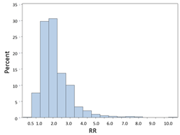
Most of the estimates are close to 2.0, the true value, but these are estimates, and sampling variability results in some estimates that are lower and some that are higher, and the distribution is skewed toward the higher values. Nevertheless, it is often possible to achieve a more normalized distribution by transforming it by taking the natural log (ln) of skewed variables like this.
If we take the natural log (ln) of the RRs or ORs, they will be more or less normally distributed as shown in the figure below. This is referred to as a log transformation, which is a useful technique for transforming a skewed variable into a reasonably normal distribution. If we were to compute the natural logarithm of the RRs obtained above, the distribution of the log transformed RRs would be much more symmetrical as shown in the figure below.
![]()
So the strategy here is to take the natural log of the observed RR or OR, then compute the upper and lower bounds of the confidence interval for the log transformed values, and then convert those values back to a regular linear scale by exponentiating them. Note that the log transformed confidence interval will be symmetrical around the point estimate, but when we convert these values back to a linear scale, the final confidence interval will be asymmetrically positioned around the point estimate.
95% Confidence Interval for a Risk Ratio
Example:
|
No CVD |
CVD |
Total |
|
|
No HTN |
1017 |
165 |
1182 |
|
HTN |
2260 |
992 |
3252 |
|
Total |
3277 |
1157 |
4434 |
[Note that this contingency table is set up in a very specific way. Outcomes are listed in the columns, and those with the outcome are in the 2nd column. Exposure status is listed in the rows with the unexposed in the 1st row. This is in preparation for getting R to do some of these calculations, as you will see a bit further along. It is set up this way because if you have summary data and need to create a contingency table in R, it will expect to see the data in this orientation. If you don't do it this way, the output will be incorrect. So, the table is set up this way here in order to make later steps easier.]
RR=CIE/CIU = (992/3252) / (165/1182) = 0.305/0.140 = 2.18
Step 1: Find the natural log of RR
> log(2.18) [1] 0.7793249
Step 2: Find the confidence limits on the natural log scale.

Step 3: Convert the upper and lower log limits back to a linear scale by exponentiating them.

We can exponentiate the limits In R by using the following commands:
> exp(0.628)
[1] 1.873859
> exp(0.930)
[1] 2.534509
Note that the confidence interval is not symmetrical with respect to the point estimate for RR.
95% Confidence Interval for an Odds Ratio
Example: (same example, but we will compute the odds ratio instead of the risk ratio)
|
No CVD |
CVD |
Total |
|
|
No HTN |
1017 |
165 |
1182 |
|
HTN |
2260 |
992 |
3252 |
|
Total |
3277 |
1157 |
4434 |
OR= (992/2260) / (165/1017) = 0.439/0.162 = 2.71
Step 1: Find the natural log of OR.
> log(2.71)
[1] 0.9969486
Step 2: Find the confidence limits on the natural log scale.

Step 3: Convert the log limits back to a linear scale by exponentiating them.

We can exponentiate them using a hand-held calculator, or Excel [=exp(0.816)], or by using R as follows:
In R:
> exp(0.816)
[1] 2.261436
> exp(1.178)
[1] 3.247872