PH717 Module 8 - Statistical Methods for Categorical Data

Introduction

Link to Video Transcript in a Word file

The previous module focused on using t-tests to comparie continuously distributed outcomes, such as body mass index, but how can you compare categorical outcomes?

This module will introduce the chi-square test of independence to test associations between categorical exposures and categorical outcomes. After completing this section you should be able to perform the chi-square test of independence by hand or using the R statistical package.

The chi-square test of independence can be used to test for differences with several types of variables that were introduced in module 1:

1. Categorical variables: Variables that fall into two or more categories that do not have any inherent ranking or ordering, such as race and ethnicity (e.g., white, black, Hispanic, Asian, etc.)
2. Dichotomous variables: Variables that have just two possible values (e.g., male or female; occupational exposure to asbestos: Yes or No; death: Yes or No; developed coronary heart disease: Yes or No)
3. Ordinal variables: Categorical variables that have more than two ranked or ordered values (e.g., physical activity: <30 minutes/week, 30-180 minutes/week, >180 minutes/week; amount of current smoking: none, <10/day, 10-20/day, 21-30/day, >30/day); or number of past heart attacks: 0, 1, 2, 3, etc.)

Essential Questions

1. How do we test the statistical significance of associations between exposures and categorical outcomes?
2. How do we determine whether an exposure increases or decreases the risk of a particular health outcome?
3. When is it most appropriate to assess data categorically?

Learning Objectives

After completing this module, you will be able to:

• Identify situations in which a chi-square test is appropriate
• Perform chi-square tests by hand and using the R computing package
• Interpret results of chi-square tests correctly
• Identify the appropriate hypothesis testing procedure for evaluating categorical data
• Communicate the results of chi-square tests for a non-technical/lay audience

A Study Using Categorical Data

People who are HIV⁺ should inform their sexual partners of their HIV status. Does the probability of doing this vary depending on mode of transmission? Researchers at Boston University School of Public Health sought to answer this question and reported their findings in the paper below.

Sexual ethics. Disclosure of HIV-positive status to partners. Stein MD, Freedberg KA, Sullivan LM, et al.: Arch Intern Med. 1998;158(3):253-7.

Abstract

"OBJECTIVE: To determine factors associated with disclosure of human immunodeficiency virus (HIV)-positive status to sexual partners.

METHODS: We interviewed 203 consecutive patients presenting for primary care for HIV at 2 urban hospitals. One hundred twenty-nine reported having sexual partners during the previous 6 months. The primary outcome of interest was whether patients had told all the sexual partners they had been with over the past 6 months that they were HIV positive. We analyzed the relationships between sociodemographic, alcohol and drug use, social support, sexual practice, and clinical variables; and whether patients had told their partners that they were HIV positive was analyzed by using multiple logistic regression.

RESULTS: Study patients were black (46%), Latino (23%), white (27%), and the majority were men (69%). Regarding risk of transmission, 41% were injection drug users, 20% were homosexual or bisexual men, and 39% were heterosexually infected. Sixty percent had disclosed their HIV status to all sexual partners. Of the 40% who had not disclosed, half had not disclosed to their one and only partner. Among patients who did not disclose, 57% used condoms less than all the time. In multiple logistic regression analysis, the odds that an individual with 1 sexual partner disclosed was 3.2 times the odds that a person with multiple sexual partners disclosed. The odds that an individual with high spousal support disclosed was 2.8 times the odds of individuals without high support, and the odds that whites or Latinos disclosed was 3.1 times the odds that blacks disclosed.

CONCLUSIONS: Many HIV-infected individuals do not disclose their status to sexual partners. Nondisclosers are not more likely to regularly use condoms than disclosers. Sexual partners of HIV-infected persons continue to be at risk for HIV transmission."

In the methods section of the paper the authors noted that they used the two independent sample t-test to test for differences in continuous variables and used two-tailed tests. They used chi-square analyses to test for differences in discrete (i.e., categorical) variables.

[Link to full article: https://jamanetwork.com/journals/jamainternalmedicine/fullarticle/191291 ]

The table below shows part of Table 1 from the paper, presenting factors associated with disclosure of HIV+ status.

The outcome is dichotomous (disclosed or did not), and the "exposure" categories are either dichotomous (two groups) or categorical (more than two categories). All of the p-values shown were computed using a chi-square test of independence.

In order to explain the chi-square (χ²) test, we will focus on the last row in the table above to determine whether the frequency of disclosing one's HIV+ status differs among injection drug users, homosexuals, and heterosexuals.

The Chi-square Test of Independence

Table – Observed Disclosure Frequency Among Subjects Posing Three Types of Transmission Risk

• The null hypothesis (H₀:) is that there is no association between HIV transmission risk group and disclosure, i.e., the frequency of disclosure does not differ across HIV transmission risk groups. 
• The alternative hypothesis (H_A:) is that there is an association between HIV transmission risk group and frequency of disclosure, i.e., that the frequency of disclosure differs across HIV transmission risk groups.

Note that the overall disclosure frequency was 77/127 = 60.6%, so the null hypothesis would predict that the disclosure frequency would be 60.6% for all three transmission modes. This was not the case; the frequency of disclosure varied from 52% to 67%. How different are these frequencies from what we would have expected under the null hypothesis (H₀:)? Could the variability have resulted from sampling error?

The chi-square test helps answer this question by calculating a test statistic (x²) based on the differences between the frequencies observed in each cell compared to the frequencies expected under the null hypothesis. The chi-square equation is:

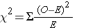
where "O" is the observed count for each exposure-outcome category, "E" is the expected count for each exposure-outcome category based on the null hypothesis, and the degrees of freedom (df) = (r-1) x (c-1), i.e., the number of rows (exposure categories) minus one times the number of columns (outcome categories) minus one in the contingency table.

If you are doing this manually, the next task is to compute the frequencies that would have been expected under the null hypothesis. If the overall frequency of disclosure was 60.6%, then H₀: would predict 60.6% exposure in all three risk categories. We can therefore compute the expected number for each category by multiplying 0.606 times the number of subjects in each exposure category. For example, for IV drug users the expected number of disclosures is 0.606 x 52 = 31.5. (It doesn't matter if these aren't whole numbers.) We can similarly multiply 0.606 times the number of subjects in the other two exposure categories as shown in the table below. The number of non-disclosures in each category is simply the category total minus the number of expected disclosures, so for the IV drug users the number of expected non-disclosures is 52 - 31.5 =  20.5.

 Table – Expected Disclosure Frequency (under H₀:) Among Subjects Posing Three Types of Transmission Risk

Next, we calculate x²:

degrees of freedom = df = (r-1)*(c-1) = (3-1)*(2-1) = 2

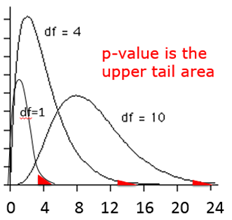
As with the t-distribution, the χ² distribution is actually a series of distributions, i.e., one for each number of degrees of freedom, and the upper tail area is the probability, i.e., the p-value. Even though it evaluates the upper tail area, the chi-square test is regarded as a two-tailed test (non-directional), since it is basically just asking if the frequencies differ.

The table below shows a portion of a table of probabilities for the chi-square distribution.

This comparison has 2 degrees of freedom, so we read across the appropriate row in the table and find that a χ²=1.95 with 2 degrees of freedom isn't even on the table. However, the p-value must be greater than 0.10, since 1.95 is clearly less than the critical value of 4.61 for an alpha level (p-value) of 0.01 with 2 degrees of freedom. Based on this we could conclude that the observed differences in frequency were not statistically significant.

We can more precisely compute the p-value using R:

> 1-pchisq(1.95,2)
[1] 0.3771924

Conclusion: This data does not provide evidence for a difference in disclosure rates. We conclude that there is no statistically significant association between HIV transmission risk category and disclosure (p-value=0.38). The proportion of HIV patients who disclose their status to sexual partners does not significantly differ across HIV transmission risk categories.

Chi-Square Analysis Using R

Analysis With Contingency Table Data

If you are given frequency data in a contingency table, you can create a data matrix to analyze the data. For example, here are the observed frequencies from the examples above.

To create the contingency table in R we would create a data object (let's arbitrarily call it "datatable") and then use the matrix function and entering the frequencies in a very specific order as shown below. First we enter the three observed counts in the first column in order and then enter the three observed counts in the the second column. We also have to specify the number of rows and the number of columns. Once we enter the data, we can check the results by simply giving the command "datatable". Lastly, we use the chisq.test function.

> datatable <- matrix(c(35,13,29,17,12,21),nrow=3,ncol=2)
> datatable
[,1] [,2]
[1,]  35   17
[2,]  13   12
[3,]  29   21
> chisq.test(datatable,correct=FALSE)

Output:

Pearson's Chi-squared test
data: datatable
X-squared = 1.8963, df = 2, p-value = 0.3875

Analysis with Raw Data from a Data Set

Alternatively, if you have raw data, you can create a contingency table from the raw data using the "table" function and then use chisq.test as shown in the example below which uses raw data from the Framingham Heart Study to look at the association between hypertension (hypert) and risk of developing coronary heart disease (chd). Note that when R creates the contingency table from raw data, it always lists the lowest alphanumeric category first. In this case the categories of hypertension are 0 (no) first and then 1 (yes). Similarly, the columns of the table list chd=0 first and chd=1 second.

>fram<-FramCHDStudy
>attach(fram)
>table(hypert,chd)
           chd
 hypert   0   1
      0 748 140
      1 380 142
> prop.table(table(hypert,chd),1)
                   chd
hypert          0         1
     0  0.8423423 0.1576577
     1  0.7279693 0.2720307

> chisq.test(table(hypert,chd),correct=FALSE)
Ouput:
Pearson's Chi-squared test
data: table(hypert, chd)
X-squared = 26.8777, df = 1, p-value = 2.168e-07

The p-value is 2.168 x 10^-7 or 0.0000002168, a very small p-value, suggesting an extremely low probabily of seeing the observed differences if the null hypothesis were true.

Conclusion:

Hypertensive adults have significantly higher risk of developing coronary heart disease (chd) compared to non-hypertensive adults (27.2% vs. 15.8%, chi-square (1 df) = 26.877, p<0.0001). [Note that when reporting results with such a small p-value, one should simplify things and simply report the difference as p<0.0001. If the p-value had been 0.0002168, we could report that as p<0.001.]

Instead of using prop.table, you can compute proportions directly in R using the math functions, e.g., the proportion of non-hypertensive adults who developed CHD = 140/(140+748) as shown below.

> 140/(140+748)
[1] 0.1576577

Test Yourself

Investigators tested a new intervention to promote smoking cessation. Among subjects exposed to the new intervention, 40/120 had quit at 6 months. Among the 80 subjects who did not receive the intervention, 10 had quit at 6 months. What was the "risk ratio" for quitting in the intervention group compared to the placebo group? Was the success rate significantly higher in the intervention group compared to the non-intervention group?

Link to Answer in a Word file

Confidence Intervals for Risk Ratios and Odds Ratios

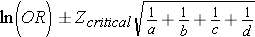
You are already familiar with risk ratios and odds ratios.

• Risk ratio [RR] = CI_e/CI_u

where CI_e=cumulative incidence in exposed (index) group and CI_u= cumulative incidence in the unexposed (reference) group

• Odds ratio [OR] =  (odds of disease in exposed) / (odds of disease in unexposed)

Both RR and OR are estimates from samples, and they are continuous measures. In order to assess the potential for random error, it is important to assess the precision of these estimates with a confidence interval, but there is a problem in that these measures are not normally distributed.

RRs and ORs can't be less than 0, but they can be infinitely greater than 0. Suppose the true RR=2.0 for a particular comparison, and we took 1,000 samples consisting of n=200 from each of two groups being compared. The distribution of RRs obtained from all of these samples might look like this:

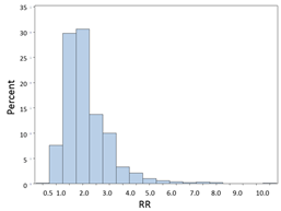
Most of the estimates are close to 2.0, the true value, but these are estimates, and sampling variability results in some estimates that are lower and some that are higher, and the distribution is skewed toward the higher values. Nevertheless, it is often possible to achieve a more normalized distribution by transforming it by taking the natural log (ln) of skewed variables like this.

If we take the natural log (ln) of the RRs or ORs, they will be more or less normally distributed as shown in the figure below. This is referred to as a log transformation, which is a useful technique for transforming a skewed variable into a reasonably normal distribution. If we were to compute the natural logarithm of the RRs obtained above, the distribution of the log transformed RRs would be much more symmetrical as shown in the figure below.

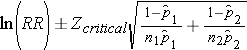
So the strategy here is to take the natural log of the observed RR or OR, then compute the upper and lower bounds of the confidence interval for the log transformed values, and then convert those values back to a regular linear scale by exponentiating them. Note that the log transformed confidence interval will be symmetrical around the point estimate, but when we convert these values back to a linear scale, the final confidence interval will be asymmetrically positioned around the point estimate.

95% Confidence Interval for a Risk Ratio

Example:

[Note that this contingency table is set up in a very specific way. Outcomes are listed in the columns, and those with the outcome are in the 2nd column. Exposure status is listed in the rows with the unexposed in the 1st row. This is in preparation for getting R to do some of these calculations, as you will see a bit further along. It is set up this way because if you have summary data and need to create a contingency table in R, it will expect to see the data in this orientation. If you don't do it this way, the output will be incorrect. So, the table is set up this way here in order to make later steps easier.]

RR=CI_E/CI_U = (992/3252) / (165/1182) = 0.305/0.140 = 2.18

Step 1: Find the natural log of RR

> log(2.18) [1] 0.7793249

Step 2: Find the confidence limits on the natural log scale.

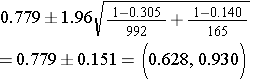
Step 3: Convert the upper and lower log limits back to a linear scale by exponentiating them.

We can exponentiate the limits In R by using the following commands:
> exp(0.628)
[1] 1.873859
> exp(0.930)
[1] 2.534509

Note that the confidence interval is not symmetrical with respect to the point estimate for RR.

95% Confidence Interval for an Odds Ratio

Example: (same example, but we will compute the odds ratio instead of the risk ratio)

OR= (992/2260) / (165/1017) = 0.439/0.162 =  2.71

Step 1: Find the natural log of OR.

> log(2.71)
[1] 0.9969486

Step 2: Find the confidence limits on the natural log scale.

Step 3: Convert the log limits back to a linear scale by exponentiating them.

We can exponentiate them using a hand-held calculator, or Excel [=exp(0.816)], or by using R as follows:

In R:

> exp(0.816)
[1] 2.261436
> exp(1.178)
[1] 3.247872

Confidence Intervals for RRs, ORs in R

The "base package" in R does not have a command to calculate confidence intervals for RRs, ORs. However, there are supplemental packages that can be loaded into R to add additional analytical tools, including confidence intervals for RR and OR. These tools are in the " epitools " package.

You must first install the package on your computer (just once), but each time you want to use it in an active R session, you need to load it.

Installing the epitools Package into R

Type the following to install the epitools package (this only needs to be done once):

>install.packages("epitools")

You should see the following message as a response in red:
Installing package into 'C:/Users/healeym/Documents/R/win-library/3.3' (as 'lib' is unspecified) trying URL 'https://cran.rstudio.com/bin/windows/contrib/3.3/epitools_0.5-7.zip' Content type 'application/zip' length 228486 bytes (223 KB) downloaded 223 KB
package 'epitools' successfully unpacked and MD5 sums checked The downloaded binary packages are in C:\Users\yourusername\AppData\Local\Temp\RtmpsLajiU\downloaded_packages

Loading the epitools Package When You Want to Use It

You only have to install the epitools package once, but you have to call it up each time you use it.

>library(epitools)
Warning message: package 'epitools' was built under R version 3.4.2

RRs and ORs from R

Situation #1: Starting with Counts from a Contingency Table:

If you are given the counts in a contingency table, i.e., you do not have the raw data set, you can re-create the table in R and then compute the risk ratio and its 95% confidence limits using the riskratio.wald() function in Epitools.

This is where the orientation of the contingency table is critical, i.e., with the unexposed (reference) group in the first row and the subjects without the outcome in the first column.
We create the contingency table in R using the matrix function and entering the data for the 1st column, then 2nd column. Note that we only enter the observed counts for each of the exposure-disease categories; we do not enter the totals in the margins. The solution in R is as follows:

Risk Ratio and Confidence Interval in R

R Code:

# The 1^stline below creates the contingency table; the 2^nd line prints the table so you can check the orientation
> RRtable<-matrix(c(1017,2260,165,992),nrow = 2, ncol = 2)
> RRtable
     [,1] [,2]
[1,] 1017  165
[2,] 2260  992
# The next line asks R to compute the RR and 95% confidence interval
> riskratio.wald(RRtable)
$data
          Outcome
Predictor  Disease1 Disease2 Total
Exposed1      1017      165  1182
Exposed2      2260      992  3252
Total         3277     1157  4434

$measure
risk ratio with 95% C.I.
Predictor  estimate    lower    upper
Exposed1 1.000000        NA     
Exposed2 2.185217 1.879441 2.540742

$p.value
two-sided
Predictor  midp.exact fisher.exact  chi.square
Exposed1          NA                  
Exposed2           0 7.357611e-31 1.35953e-28zz

$correction [1] FALSE

attr(,"method") [1] "Unconditional MLE & normal approximation (Wald) CI"

The risk ratio and 95% confidence interval are listed in the output under $measure.

Odds Ratio and 95% Confidence Interval in R

Case-control studies use an odds ratio as the measure of association, but this procedure is very similar to the analysis above for RR.

> ORtable<-matrix(c(1017,2260,165,992),nrow = 2, ncol = 2)
> ORtable
     [,1] [,2]
[1,] 1017  165
[2,] 2260  992
> oddsratio.wald(ORtable)
$data
          Outcome
Predictor  Disease1 Disease2 Total
 Exposed1     1017      165  1182
 Exposed2     2260      992  3252
 Total        3277     1157  4434

$measure
odds ratio with 95% C.I.
Predictor  estimate    lower    upper
Exposed1 1.000000        NA     
Exposed2 2.705455 2.258339 3.241093

$p.value two-sided
Predictor  midp.exact fisher.exact  chi.square
Exposed1          NA                  
Exposed2           0 7.357611e-31 1.35953e-28

$correction [1] FALSE

attr(,"method")
[1] "Unconditional MLE & normal approximation (Wald) CI"

Situation #2: Starting with Counts from a Raw Data Set:

If you have a raw data set, computing risk ratios and odds ratios and their corresponding 95% confidence intervals is even easier, because the contingency table can be created using the table() command instead of the matrix function.

For example, if I have data from the Framingham Heart Study and I want to compute the risk ratio for the association between type 2 diabetes and risk of being hospitalized with a myocardial infarction, I first use the table() command.

> table(diabetes,hospmi)

              hospmi

diabetes       0       1

            0 2557   210

            1 183     48

Then, to compute the risk ratio and confidence limits, I insert the table parameters into the riskratio.wald() function:

> riskratio.wald(table(diabetes,hospmi))

$data

              hospmi

diabetes       0     1 Total

    0         2557 210   2767

    1         183   48   231

    Total 2740 258   2998

$measure

              risk ratio with 95% C.I.

diabetes estimate       lower     upper

            0   1.00000   NA       NA

            1   2.73791 2.062282 3.63488

 Using the same data, I can similarly compute an odds ratio and its confidence interval using the oddsratio.wald()function:

> oddsratio.wald(table(diabetes,hospmi))

$data

              hospmi

diabetes       0     1 Total

    0         2557 210  2767

    1          183   48   231

    Total 2740 258  2998

$measure

              odds ratio with 95% C.I.

diabetes estimate       lower      upper

            0 1.000000   NA       NA

            1 3.193755 2.256038 4.521233

  Note that, since this is a cohort study, it makes sense to compute the risk ratio, but I also have the option of computing an odds ratio, although in a case-control study one can only calculate an odds ratio. Notice also that in the example above, the odds ratio was somewhat more extreme than the risk ratio.

Test Yourself

Problem #1

A clinical trial was conducted to compare a new blood pressure-lowering medication to a placebo. Patients were enrolled and randomized to receive either the new medication or a placebo. The data below were collected at the end of the 6 week study.

Generate a point estimate and 95% confidence interval for the risk ratio of side effects in patients assigned to the experimental group as compared to placebo. Use both the hand calculation method and the method using R to see if you get the same answers. Interpret the results in a sentence or two.

Problem #2

The table below summarizes parental characteristics for children of normal weight and children classified as overweight or obese. Perform a chi-square test by hand to determine if there is an association between the mother's BMI and the child's weight status. Compute the p-value and report your conclusion.

 Link to Answer in a Word file

An Exercise Using R to Compute Chi-Squared from a Data Set

In this exercise you will examine associations between baseline health characteristics measured during the 1^st  visit in the Framingham Heart Study and development of heart disease & death over 20 years of follow-up. You will use a subset (n=500) of the data saved in the file FramHSn500.csv.

The data is coded as shown in the table below:

 Save your R code and output as you answer the following questions.

1. Are smokers at higher risk of death over follow-up than non-smokers?  Test this with a chi-square test, reporting the proportion of smokers and non-smokers who have died over 20 years of follow-up, the risk ratio, the value of the chi-square statistic, degrees of freedom, and p-value.  Summarize your conclusions.
2. Are smokers at higher risk of death over follow-up than non-smokers?  Find the risk ratio of death for smokers vs. non-smokers, and the 95% confidence interval for this risk ratio (remember that the orientation of the table matters when finding a RR).  Given this confidence interval, do smokers have significantly higher risk of death?  Explain.
3.  Is there an association between coffee consumption and death over the 20-year follow-up?  Test this with a chi-square statistic, reporting the proportion who have died in each category of coffee consumption, the value of the test statistic, degrees of freedom, and p-value. Summarize your conclusions.
4. Do those who develop heart disease have a higher risk of death over follow-up?  What percent of those with and without heart disease die over follow-up?  Test through a chi-square statistic, reporting the value of the test statistic, degrees of freedom, and p-value.  Summarize your conclusions.
5. Do those who develop heart disease have a higher risk of death over follow-up?  Find the risk ratio of death for with vs. without heart disease, and the 95% confidence interval for this relative risk (remember that the orientation of the table matters when finding a RR).  Given this confidence interval, do those who develop heart disease have significantly higher risk of death?  Explain.

Link to All Answers in a Word file

Test Yourself

#1 - Starship Enterprise

Now let's return to the question of mortality rates on the Enterprise. Here is the data. Is the mortality rate significantly greater among the Red crew members? Use R to analyze these data.

#2 - The Titanic

Now let's reconsider 1st, 2nd, or 3rd class passengers differed significantly in their risk of death after the Titanic struck an iceberg. Here is the data.

Use R to compute the risk ratio of death for 2nd class compared to 1st class (reference group) and for 3rd class compared to 1st class. Also compute the 95% confidence intervals for these risk ratio estimates and the p-values.

Was the risk of death significantly higher in 2nd class and 3rd class passengers?