


Useful Tips
Creating a New Dichotomous Variable from a Continuous Measure
Example: Child verbal IQ (continuous measure)
In this example, "verbiq" is the name of a continuous variable measuring verbal IQ score. We wish to create a new categorical indicating subjects with low verbal IQ scores, i.e., less than 75. We will create a new variable called "low-iq" which will have a value of 1 if verbiq < 75 and a value of 0 if verbiq is 75 or greater.
> lowiq <- ifelse(verbiq<75,1,0)
The ifelse statement tells R to assign a subject a "1" if verbal IQ is less than 75; else assign a subject a "0" (which means that verbiq must be greater than or equal to 75).
> table(lowiq)
> lowiq
0 1
467 133
The table confirms that the new dichotomous variable is coded correctly.
Creating a Side-by-Side Boxplot
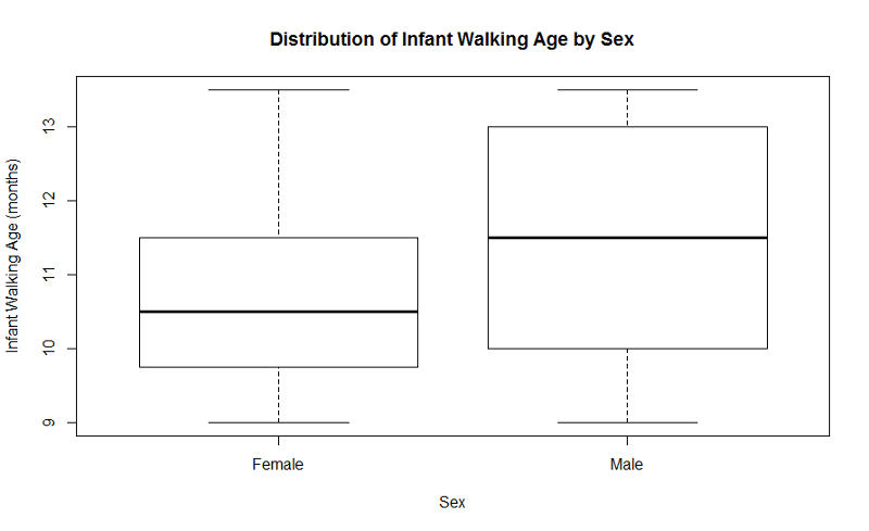
Example: Producing a side-by-side boxplot for the age at which an infant could walk comparing male to female infants.
"Sexmale" was coded as "1" for males and "0" for females. The continuous outcome, "Agewalk", is the age in months that the infant could walk.
> boxplot(Agewalk~Sexmale,names=c("Female","Male"),
main="Distribution of Infant Walking Age by Sex",
xlab="Sex",ylab="Infant Walking Age (months)")
Creating Side-by-Side Bar Charts
Example: Producing grouped bar charts for whether an infant could walk by 1 year of age (outcome) stratified by sex (exposure).
"Sexmale" was coded as "1" for males and "0" for females. The dichotomous outcome, "By1year", is an indicator variable, where "1" indicated that the infant could walk by 1 year and "0" indicated that the infant could not walk by 1 year.
> barplot(table(By1year,Sexmale),beside=TRUE,
names=c("Females","Males"),col=c("blue","green"))
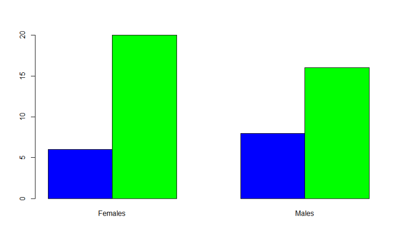
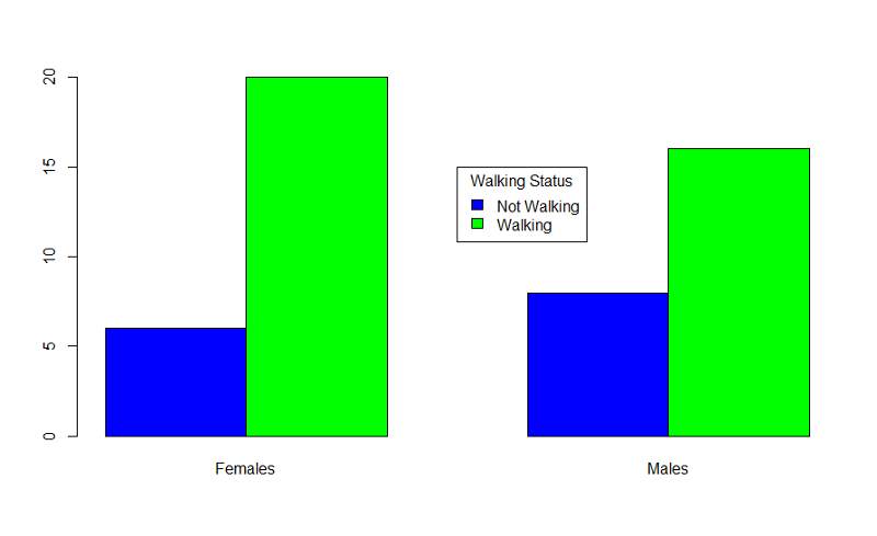
In the table statement, the first variable is the outcome plotted on the y axis, the exposure is the second variable. If you want to add a legend, you could use the following code:
> barplot(table(By1year,Sexmale),beside=TRUE,
names=c("Females","Males"),col=c("blue","green"))
> legend(x=3.5,y=15,legend=c("Not Walking","Walking"),fill=c("blue","green"),
title="Walking Status")
95% Confidence Interval for the Difference in Proportions
Example: Proportion of infants walking by 11 months of age according to infant exercise program. "walkby11" is the name of a dichotomous outcome variable for which "1"=walking by 11 months and "0"=not walking by 11 months, and "exercise" is a dichotomous exposure variable, for which "2"=assigned to exercise intervention and "1"=assigned to usual care
To find the 95% CI for a difference in proportions:
> table(Walkby11,Exercise)
Exercise
Walkby11 1 2
0 13 14
1 20 3
The table helps to present the data so that you can identify the correct cells for the prop.test command
> prop.test(c(20,3),c(33,17),correct=TRUE)
2-sample test for equality of proportions with continuity correction
data: c(20, 3) out of c(33, 17)
X-squared = 6.6961, df = 1, p-value = 0.009662
alternative hypothesis: two.sided
95 percent confidence interval:
0.1387907 0.7203893
sample estimates:
prop 1 prop 2
0.6060606 0.1764706
In prop.test, we concatenate values: first, the number of outcome successes (walkby11=1) among non-exercises compared to exercisers: c(20,3); and second the total number of non-exercisers (13+20) compared to exercisers (14+3): c(33,17). Since one cell has only 3 events (exercisers who walk by 11 months), we state the correct=TRUE; if all cells have at least 5 subjects, then correct=FALSE.
The 95% CI is (0.139, 0.720) or (13.9%, 72.0%). The difference in proportions is 0.606-0.1765=0.43.