PH717 Introduction to R Statistical Programming
The Framingham Heart Study (FHS) began in 1948 when investigators enrolled 5,209 men and women aged 30-62 from Framingham, Massachusetts. Subjects provided baseline information on many variables, and they returned to the study office every two years for a detailed medical history, physical examination, and lab tests. They also monitored the cohort carefully and recorded adverse health outcomes, focusing primarily on cardiovascular diseases. In 1971 they enrolled a second cohort consisting of the offspring cohort of the initial cohort, and in 2002 they enrolled a third cohort consisting of the grandchildren of the original cohort. The data that was collected, and the many subsequent analyses that have been conducted led to the identification of the major risk factors for cardiovascular disease: high blood pressure, high blood cholesterol, smoking, obesity, diabetes, physical inactivity, and many other risk factors.
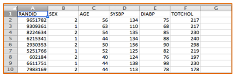
One can think of the data collected in the Framingham study and others as a series of tables with many variables (demographic information, exposures and outcomes) in the columns and each subject listed on a separate row. The figure below shows a portion of an Excel spreadsheet that was used to download the first 10 subjects in a very small subset of the FHS data. There is a random identification number in the first column, and columns indicating each subject's sex, age in years, systolic blood pressure, and total cholesterol. There are many more variables, but this small subset gives you an idea of the structure of a data set.
Excel spreadsheets can be used to collect and store tables of data of this type, and Excel can also be used for a variety of simple statistical tests. For example, Excel can perform chi-squared tests, t-tests, correlations, and simple linear regression. However, it has a number of limitations. Public health researchers and practitioners frequently perform more complex analyses, such as multiple linear regression and multiple logistic regression, which cannot be performed in Excel, so it is useful to become familiar with more sophisticated packages like R.
[NOTE: An online learning module is available for students who would like to learn to use Excel at Using Spreadsheets - Excel & Numbers]
One key advantage to collecting or importing data into Excel is that the data can then be saved as a .CSV file, that is as a "comma-separated values" file that can easily be imported into the R statistical package. We will be using a number of data files that have been saved as .CSV files for this course.
The R statistical package is a powerful open-source program that is free. It will allow you to perform all of the necessary statistical procedures for this course, and it will likely be useful to many of you for professional projects. In addition, R will enable you to produce excellent graphics (even better than those produced with SAS).
This exercise will introduce you to using R, even if you have no prior experience. The exercise will walk you through how to install R, how to import data sets, and how to analyze your data.
You will first install the base system for R and then install the RStudio, which provides a much more user-friendly interface.
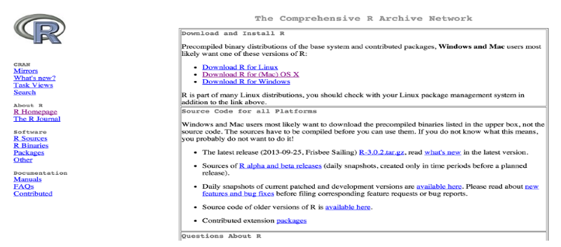
In your browser go to https://cran.r-project.org/
Select Download R for Mac or for Windows
In your browser go to https://www.rstudio.com/products/rstudio/

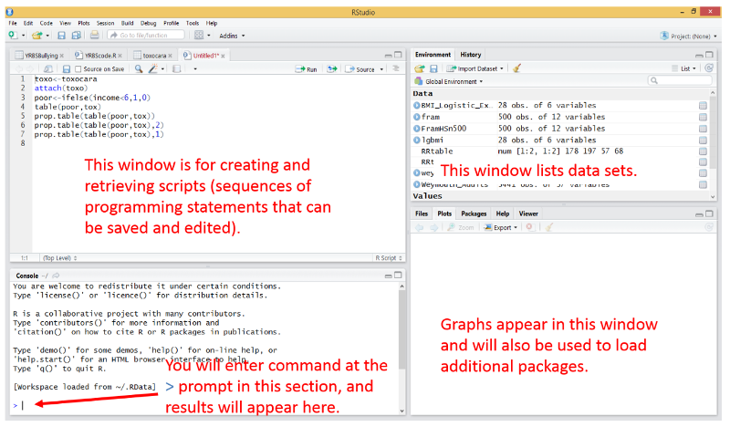
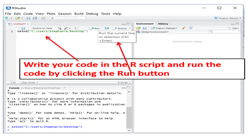
Once the RStudio is installed, it will have several windows as shown in the image below.
The modules for this course have many examples of how to use R for specific tasks, and you will be using these from week to week. The examples embedded into each week's learning modules will provide you with all of the necessary instructions for using R in this course, and it shouldn't be necessary to seek other instruction. However, if you wish to learn more about R, here are links to additional resources.
All data sets used in PH717 are comma separated value (.csv) files. For example, in this session we will be importing two data set files:
.csv files are like spreadsheets, but are saved in a simpler format that makes it possible for R to read them. If we want to create our own data set, we could enter the data into an Excel spreadsheet and save it as a .csv using "Save as" to save it in a .CSV format.
For the exercise below:
Try entering the following commands in the R Console at the lower left window. You do not have to enter the comments in green. Just enter the commands in blue and hit ?Enter?. You should see the result written in black after the [1].
# Addition
> 7+3
[1] 10
# Subtraction
> 7-3
[1] 4
# Multiplication
> 8*7
[1] 56
#Division
> 100/50
[1] 2
# Square root
> sqrt(81)
[1] 9
# Exponents
> 9^2
[1] 81
The 10 minute video below walks you through using R Studio to import a data set and create and execute a script to analyze it.
Now try it yourself. First, download the framstudy.csv data set onto your local computer. Then import the data set into R. There are two ways to do this.
The easiest way is to click on the "Import Data set" button at the upper right in the RStudio console and then browse your computer and follow the instructions. If the dialog asks if the data set has a header, say "yes", since this data set and others for this course have headers (i.e., titles) for their columns.
Once the file has been imported, we usually give it a short nickname to cut down on typing:
> fram <- framstudy
"fram" is a short name or a nickname that I made up for the data set to reduce typing during programming. The "less than" character followed by a dash (<- ) looks a bit like an arrow and functions as an assigner to tell R that we are assigning a name to a data set we are importing.
You can also use the traditional R command below as an alternative.
> fram <- read.csv(file.choose()) and then click "Run" or hit the "Enter" key.
> read.csv(file.choose()) is a function, a set of hard-coded instructions that tells R how to complete a task, e.g., how to open and read a chosen csv file.
Attach the Data Set
Once the data set has been imported, you should "attach" the data so that R defaults to performing actions on this particular data set.
> attach(fram)
If you finish with an attached data set and want to work with another data set, you should detach the first one [ > detach(fram)] and then attach the new one.
View the Data Set in R
> View(fram) [Then hit the enter key or click on the ?Run? tab to execute the command]
View() is a function that tells R to open a new window so that we can look at the data set.
Note that the View command uses an uppercase "V".
To view the data you can also just click on the data set name in the upper right window.
Once you have imported the data set, it will be listed in the "Environment" tab in the window at the upper right. If you have a large data set, it is better to just click on the small blue arrow next to the data set name in the Environment section to view it.
Writing Code in R - Important Notes
You can execute code one step at a time in the console (lower left window), and this is useful for quick one step math calculations, but it is usually more convenient to list all of your coding statements in a script in the window at the upper left and then saving the script for future use. When you enter code into the script window at the upper left, do not begin the line with a > character. You can also execute the code from the script editing window by clicking on the "Run" tab at the top of the editing window. To save a script, click on the "File" tab at the upper left and select either Save as or Save.
To start a new script, click on the File tab, then on New File, then on R Script.
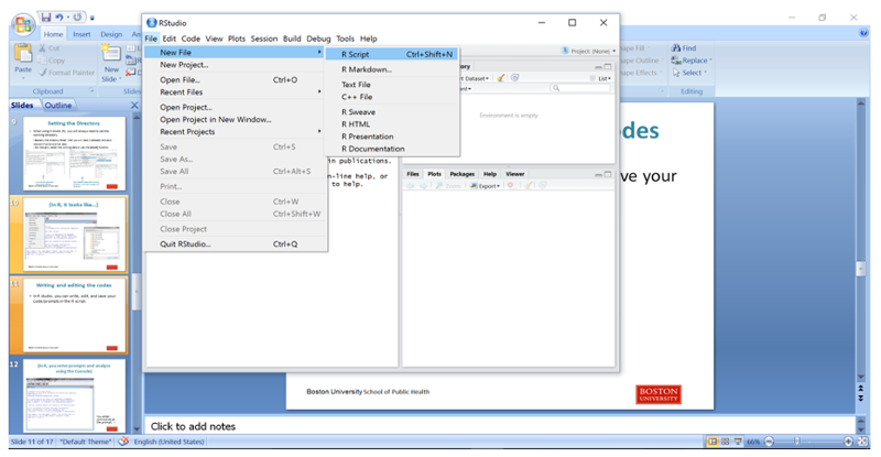
Then type in your coding statements.
Here is a short sample script:
# (A comment) Import the framstudy.csv file and call it "fram"
########################
fram<-framstudy
# Next attach the file to tell R it is the "go to" file (the default)
attach(fram)
View(fram)
# Determine the mean, median, and distribution of continuous variables
quantile(AGE)
summary(AGE)
# Determine the number and proportion of males and females
table(SEX)
prop.table(table(SEX))
# Make a mistake in naming a variable (case)
summary(Age)
Enter the script above into the R editor and save it as follows:
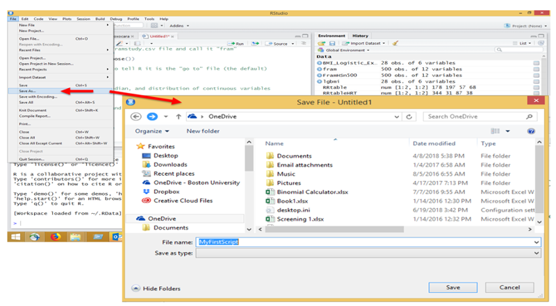
Then execute the script by hitting the "Run" tab repeatedly in the editor. When you get to the "View(fram)" step, the editor will show the data file, but you can return to the script by clicking on the tab for the script at the top of the window.
The output from the executed script will appear in the Console window at the lower left, and it should look like this:
> fram<- framstudy
> attach(fram)
> View(fram)
> quantile(AGE)
0% 25% 50% 75% 100%
39 45 52 59 65
> summary(AGE)
Min. 1st Qu. Median Mean 3rd Qu. Max.
39.00 45.00 52.00 52.41 59.00 65.00
> table(SEX)
SEX
1 2
19 30
> prop.table(table(SEX))
SEX
1 2
0.3877551 0.6122449
> summary(Age)
Error in summary(Age) : object 'Age' not found
Note that there was an error message because we gave the command "summary(Age)", but the variable for age is all upper case (AGE), so R did not find it.
In 2003-2004 Weymouth conducted a town-wide health survey, the results of which raised concerns about the general health of the residents. The data set below is a subset of the actual data that was collected and analyzed by John Snow, Inc.
First, open the Weymouth data set from this link: WeymouthSurveyData.csv
Save the data set to your computer. Then load the data set into R either be using the import data set function or by using the command
Begin a new script in the RStudio editor with the following code:WeymouthSurveyData <- read.csv(file.choose())
### Part 1###
# The first command below creates a data frame object called 'wey'. This is a short nickname for the data set.
wey<-WeymouthSurveyData
# Next, attach the data set
attach(wey)
# Create a derived variable for the respondent's age in 2002 (when the data was collected) based on their reported birth year.
age=(2002-birth_yr)
# Compute body mass index (BMI) as shown below.
bmi=weight/(hgt_inch)^2*703
# Compute the mean and standard deviation of bmi and quantiles
mean(bmi)
[1] 26.62516
sd(bmi)
[1] 5.257648
quantile(bmi)
0% 25% 50% 75% 100%
3.719577 23.052515 25.799445 29.190311 54.548669
summary(bmi)
Min. 1st Qu. Median Mean 3rd Qu. Max.
3.72 23.05 25.80 26.63 29.19 54.55
The next page continues the exercise with code that produces histograms and boxplots.
# Make a histogram of the age distribution
hist(age)

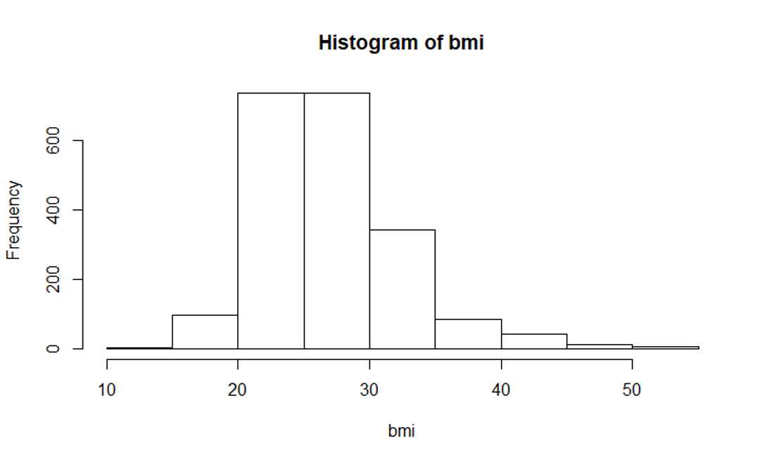
# Make a histogram and a boxplot of bmi
hist(bmi)
Next
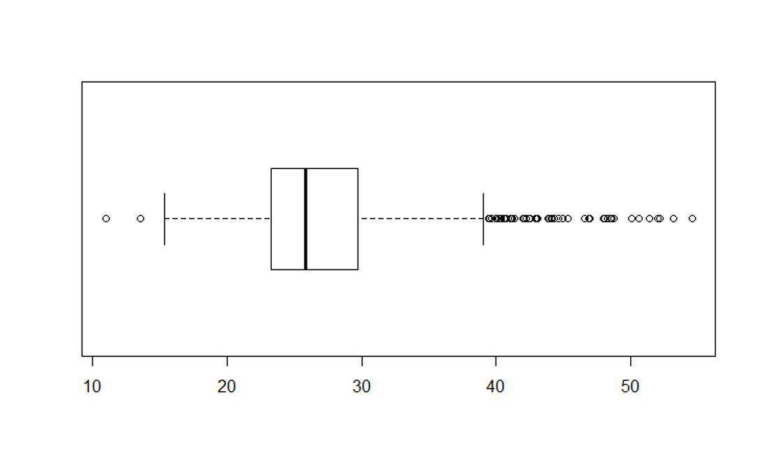
boxplot(bmi)
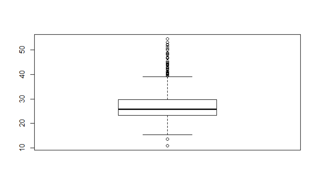
# Next, modify the boxplot to a horizontal orientation
boxplot(bmi, horizontal = TRUE)
# Modify the BMI histogram with the code below
hist(bmi, main="BMI Distribution in Weymouth Adults",
xlab = "BMI", border="blue", col="green", xlim=c(10,50),
las=1, breaks=8)

Once you have everything working, save your script for future reference. You will be using these coding functions throughout the course.
Example: Child verbal IQ (continuous measure)
In this example, "verbiq" is the name of a continuous variable measuring verbal IQ score. We wish to create a new categorical indicating subjects with low verbal IQ scores, i.e., less than 75. We will create a new variable called "low-iq" which will have a value of 1 if verbiq < 75 and a value of 0 if verbiq is 75 or greater.
> lowiq <- ifelse(verbiq<75,1,0)
The ifelse statement tells R to assign a subject a "1" if verbal IQ is less than 75; else assign a subject a "0" (which means that verbiq must be greater than or equal to 75).
> table(lowiq)
> lowiq
0 1
467 133
The table confirms that the new dichotomous variable is coded correctly.
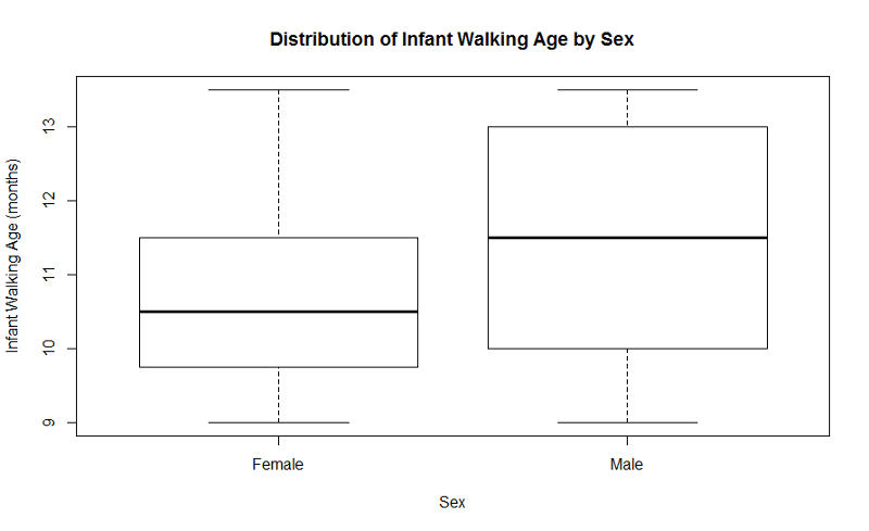
Example: Producing a side-by-side boxplot for the age at which an infant could walk comparing male to female infants.
"Sexmale" was coded as "1" for males and "0" for females. The continuous outcome, "Agewalk", is the age in months that the infant could walk.
> boxplot(Agewalk~Sexmale,names=c("Female","Male"),
main="Distribution of Infant Walking Age by Sex",
xlab="Sex",ylab="Infant Walking Age (months)")
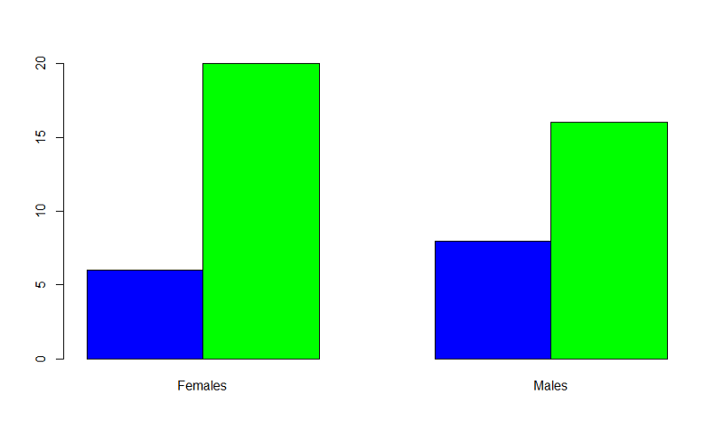
Example: Producing grouped bar charts for whether an infant could walk by 1 year of age (outcome) stratified by sex (exposure).
"Sexmale" was coded as "1" for males and "0" for females. The dichotomous outcome, "By1year", is an indicator variable, where "1" indicated that the infant could walk by 1 year and "0" indicated that the infant could not walk by 1 year.
> barplot(table(By1year,Sexmale),beside=TRUE,
names=c("Females","Males"),col=c("blue","green"))
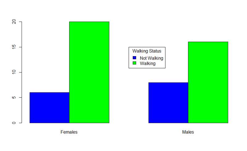
In the table statement, the first variable is the outcome plotted on the y axis, the exposure is the second variable. If you want to add a legend, you could use the following code:
> barplot(table(By1year,Sexmale),beside=TRUE,
names=c("Females","Males"),col=c("blue","green"))
> legend(x=3.5,y=15,legend=c("Not Walking","Walking"),fill=c("blue","green"),
title="Walking Status")
Example: Proportion of infants walking by 11 months of age according to infant exercise program. "walkby11" is the name of a dichotomous outcome variable for which "1"=walking by 11 months and "0"=not walking by 11 months, and "exercise" is a dichotomous exposure variable, for which "2"=assigned to exercise intervention and "1"=assigned to usual care
To find the 95% CI for a difference in proportions:
> table(Walkby11,Exercise)
Exercise
Walkby11 1 2
0 13 14
1 20 3
The table helps to present the data so that you can identify the correct cells for the prop.test command
> prop.test(c(20,3),c(33,17),correct=TRUE)
2-sample test for equality of proportions with continuity correction
data: c(20, 3) out of c(33, 17)
X-squared = 6.6961, df = 1, p-value = 0.009662
alternative hypothesis: two.sided
95 percent confidence interval:
0.1387907 0.7203893
sample estimates:
prop 1 prop 2
0.6060606 0.1764706
In prop.test, we concatenate values: first, the number of outcome successes (walkby11=1) among non-exercises compared to exercisers: c(20,3); and second the total number of non-exercisers (13+20) compared to exercisers (14+3): c(33,17). Since one cell has only 3 events (exercisers who walk by 11 months), we state the correct=TRUE; if all cells have at least 5 subjects, then correct=FALSE.
The 95% CI is (0.139, 0.720) or (13.9%, 72.0%). The difference in proportions is 0.606-0.1765=0.43.