


One-Sample Tests
Suppose we have a single sample. The questions we might want to answer are:
- What is the mean value?
- Is the mean value significantly different from a given or theoretic value?
A one-sample test compares the mean from one sample to a hypothesized value that is pre-specified in your null hypothesis.
Parametric One-sample T-test
Boston Data and Assumption Checking
A one-sample t-test is a parametric test, which is based on the normality and independence assumptions (in probability jargon, "IID": independent, identically-distributed random variables). Therefore, checking these assumptions before analyzing data is necessary.
We will use is the Boston Housing Data, which includes several potential explanatory variables, and the general question of what factors determine housing values (well, at least in Boston 1970!) is of interest. It contains 506 census tracts in the Boston Standard Statistical Metropolitan Area (SMSA) in 1970. This dataset is available within the MASS library and can be access via the name Boston. Here is a description of the dataset:
|
Variable Name |
Description |
|
crim |
Per capita crime rate by town |
|
zn |
Proportion of residential land zoned |
|
indus |
Proportion of non-retail business acres per town |
|
chas |
Charles River dummy variable (1 if tract bounds river, 0 otherwise) |
|
nox |
nitrogen oxide concentration (parts per 10 million) |
|
rm |
average number of rooms per dwelling |
|
age |
proportion of owner-occupied units built prior to 1940 |
|
dis |
weighted mean of distances to five Boston employment centers |
|
rad |
index of accessibility to radial highways |
|
tax |
full-value property-tax rate per $10,000 |
|
ptratio |
pupil-teacher ratio by town |
|
black |
1000(Bk-0.63)^2 where Bk is the proportion of blacks by town |
|
lstat |
lower status of the population (percent) |
|
medv |
median value of owner-occupied homes in $1000s |
> library(MASS)
> help(Boston)
> attach(Boston)
As usual, we begin with a set of single sample plots along with some summary statistics.
> summary(rm)
Min. 1st Qu. Median Mean 3rd Qu. Max.
3.561 5.886 6.208 6.285 6.623 8.780
This summary() function gives us six pieces of information about our variable rm. The mean and median are close to each other and so we expect the variable rm is more likely symmetric. Here are some plots to look more closely at these data.
> par(mfrow=c(2,2))
> plot(rm)
> hist(rm, main= "Histogram of number of Rooms")
> qqnorm(rm, main= "QQ-plot for number of Rooms")
> qqline(rm)
> boxplot(rm)

Alternatively, we may conduct a formal test, the Shapiro-Wilk test, to see whether the data come from a normal distribution.
- H0: The data are sampled from a normal distribution
- H1: The data are not sampled from a normal distribution.
A small significant p-value (< 0.05), as shown below, means that we reject the null hypothesis (and conclude that the data is probably not normally distributed).
> shapiro.test(rm)
Shapiro-Wilk normality test
data: rm
W = 0.9609, p-value = 2.412e-10
We see that we reject the null hypothesis that the rm variable was sampled from a normal distribution (W = 0.9609, p-value = 2.412e-10).
The next assumption is independence. In this case, the data were collected from different census tracts and we assume that each census tract is independent from each other, and hence the number of rooms can be assumed to be independent as well.
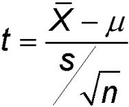
One-sample t-test for the mean μ
Suppose we are interested in testing whether the average number of rooms per dwelling in Boston in 1970 equals 6. The assumptions for a one-sample t-test are:
- Independent observations
- Sample drawn from a Normal distribution
|
Test Statistic (image from Wikipedia) |
|
|
|
|
We can use t.test() function in R. R performs a two-tailed test by default, which is what we need in our case.
> t.test(rm, mu=6)
One Sample t-test
data: rm
t = 9.1126, df = 505, p-value < 2.2e-16
alternative hypothesis: true mean is not equal to 6
95 percent confidence interval:
6.223268 6.346001
sample estimates:
mean of x
6.284634
- H0: The mean of the number of rooms per dwelling is equal to 6
- Ha: The mean of the number of rooms per dwelling is not equal to 6
The point estimate of the population mean is 6.28, and the 95% confidence interval is from 6.223 to 6.346. The hypothesis testing p-value is smaller than 0.05 ( <2.2e-16, t = 9.11 with df = 505), which leads us to reject the null hypothesis that the mean number of rooms per dwelling is equal to 6. Thus, we conclude that the average number of rooms per dwelling in Boston does not equal 6. (That's all we can say given our hypothesis!)
|
Location, location, location! People are always concerned about location while looking for a home. Suppose we are interested in the weighted distance to five Boston employment centers and would like to know if the average distance is around 3.5 miles.
(a) Conduct a t-test for testing whether the average distance is around 3.5. (b) What is the mean and median distance? (c) Is the distance normally distributed? Use plots and a formal normality test to decide. (d) Is the one-sample t-test appropriate for these data? |

One-Sample t Test in R (R Tutorial 4.1) MarinStatsLectures [Contents ]
]
![]()
![]()
Non-parametric Wilcoxon Signed-Rank Test
A quick overview of parametric vs. nonparametric testing: http://www.mayo.edu/mayo-edu-docs/center-for-translational-science-activities-documents/berd-5-6.pdf
What do we do if the normality assumption fails? Here is where the non-parametric test comes in. The Wilcoxon Signed rank test can compare the median to a hypothesized median value. For example, in our case,
> wilcox.test(dis, mu=3.5)
Wilcoxon signed rank test with continuity correction
data: dis
V = 67110, p-value = 0.3661
alternative hypothesis: true location is not equal to 3.5
- H0: The median weighted distance is equal to 3.5
- Ha: The median weighted distance is not equal to 3.5
We fail to reject the null hypothesis that the median weighted distance is equal to 3.5 (V = 67110, p-value = 0.3661).
The wilcox.test() function conducts a two-sided test by default but a one-sided test is also available by changing the alternative argument. The alternative = "less" command would test the null hypothesis that the median weighted distance is less than 3.5, the alternative = "greater" command would test the null hypothesis that the median weighted distance is more than 3.5. The output for wilcox.test() is compact but other information such as confidence intervals can be requested if necessary. Note that the Wilcoxon signed-rank test still assumes independence, although it relaxes the normality assumption.
wilcox.test(dis, mu = 3.5, alternative="less")
wilcox.test(dis, mu=3.5, alternative= "greater")
|
|
Mann Whitney U (aka Wilcoxon Rank-Sum) Test in R (R Tutorial 4.3) MarinStatsLectures [Contents]
![]()
![]()
