One and Two Sample Tests and ANOVA
Table of Contents»
Ching-Ti Liu, PhD, Associate Professor, Biostatistics
Jacqueline Milton, PhD, Clinical Assistant Professor, Biostatistics
Avery McIntosh, doctoral candidate
This module will show you how to conduct basic statistical tests in R:
By the end of this session students will be able to:
Suppose we have a single sample. The questions we might want to answer are:
A one-sample test compares the mean from one sample to a hypothesized value that is pre-specified in your null hypothesis.
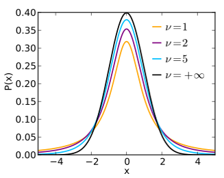
A one-sample t-test is a parametric test, which is based on the normality and independence assumptions (in probability jargon, "IID": independent, identically-distributed random variables). Therefore, checking these assumptions before analyzing data is necessary.
We will use is the Boston Housing Data, which includes several potential explanatory variables, and the general question of what factors determine housing values (well, at least in Boston 1970!) is of interest. It contains 506 census tracts in the Boston Standard Statistical Metropolitan Area (SMSA) in 1970. This dataset is available within the MASS library and can be access via the name Boston. Here is a description of the dataset:
|
Variable Name |
Description |
|
crim |
Per capita crime rate by town |
|
zn |
Proportion of residential land zoned |
|
indus |
Proportion of non-retail business acres per town |
|
chas |
Charles River dummy variable (1 if tract bounds river, 0 otherwise) |
|
nox |
nitrogen oxide concentration (parts per 10 million) |
|
rm |
average number of rooms per dwelling |
|
age |
proportion of owner-occupied units built prior to 1940 |
|
dis |
weighted mean of distances to five Boston employment centers |
|
rad |
index of accessibility to radial highways |
|
tax |
full-value property-tax rate per $10,000 |
|
ptratio |
pupil-teacher ratio by town |
|
black |
1000(Bk-0.63)^2 where Bk is the proportion of blacks by town |
|
lstat |
lower status of the population (percent) |
|
medv |
median value of owner-occupied homes in $1000s |
> library(MASS)
> help(Boston)
> attach(Boston)
As usual, we begin with a set of single sample plots along with some summary statistics.
> summary(rm)
Min. 1st Qu. Median Mean 3rd Qu. Max.
3.561 5.886 6.208 6.285 6.623 8.780
This summary() function gives us six pieces of information about our variable rm. The mean and median are close to each other and so we expect the variable rm is more likely symmetric. Here are some plots to look more closely at these data.
> par(mfrow=c(2,2))
> plot(rm)
> hist(rm, main= "Histogram of number of Rooms")
> qqnorm(rm, main= "QQ-plot for number of Rooms")
> qqline(rm)
> boxplot(rm)

Alternatively, we may conduct a formal test, the Shapiro-Wilk test, to see whether the data come from a normal distribution.
A small significant p-value (< 0.05), as shown below, means that we reject the null hypothesis (and conclude that the data is probably not normally distributed).
> shapiro.test(rm)
Shapiro-Wilk normality test
data: rm
W = 0.9609, p-value = 2.412e-10
We see that we reject the null hypothesis that the rm variable was sampled from a normal distribution (W = 0.9609, p-value = 2.412e-10).
The next assumption is independence. In this case, the data were collected from different census tracts and we assume that each census tract is independent from each other, and hence the number of rooms can be assumed to be independent as well.
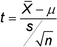
Suppose we are interested in testing whether the average number of rooms per dwelling in Boston in 1970 equals 6. The assumptions for a one-sample t-test are:
|
Test Statistic (image from Wikipedia) |
|
|
|
|
We can use t.test() function in R. R performs a two-tailed test by default, which is what we need in our case.
> t.test(rm, mu=6)
One Sample t-test
data: rm
t = 9.1126, df = 505, p-value < 2.2e-16
alternative hypothesis: true mean is not equal to 6
95 percent confidence interval:
6.223268 6.346001
sample estimates:
mean of x
6.284634
The point estimate of the population mean is 6.28, and the 95% confidence interval is from 6.223 to 6.346. The hypothesis testing p-value is smaller than 0.05 ( <2.2e-16, t = 9.11 with df = 505), which leads us to reject the null hypothesis that the mean number of rooms per dwelling is equal to 6. Thus, we conclude that the average number of rooms per dwelling in Boston does not equal 6. (That's all we can say given our hypothesis!)
|
Location, location, location! People are always concerned about location while looking for a home. Suppose we are interested in the weighted distance to five Boston employment centers and would like to know if the average distance is around 3.5 miles.
(a) Conduct a t-test for testing whether the average distance is around 3.5. (b) What is the mean and median distance? (c) Is the distance normally distributed? Use plots and a formal normality test to decide. (d) Is the one-sample t-test appropriate for these data? |
One-Sample t Test in R (R Tutorial 4.1) MarinStatsLectures [Contents]
A quick overview of parametric vs. nonparametric testing: http://www.mayo.edu/mayo-edu-docs/center-for-translational-science-activities-documents/berd-5-6.pdf
What do we do if the normality assumption fails? Here is where the non-parametric test comes in. The Wilcoxon Signed rank test can compare the median to a hypothesized median value. For example, in our case,
> wilcox.test(dis, mu=3.5)
Wilcoxon signed rank test with continuity correction
data: dis
V = 67110, p-value = 0.3661
alternative hypothesis: true location is not equal to 3.5
We fail to reject the null hypothesis that the median weighted distance is equal to 3.5 (V = 67110, p-value = 0.3661).
The wilcox.test() function conducts a two-sided test by default but a one-sided test is also available by changing the alternative argument. The alternative = "less" command would test the null hypothesis that the median weighted distance is less than 3.5, the alternative = "greater" command would test the null hypothesis that the median weighted distance is more than 3.5. The output for wilcox.test() is compact but other information such as confidence intervals can be requested if necessary. Note that the Wilcoxon signed-rank test still assumes independence, although it relaxes the normality assumption.
wilcox.test(dis, mu = 3.5, alternative="less")
wilcox.test(dis, mu=3.5, alternative= "greater")
|
|
Mann Whitney U (aka Wilcoxon Rank-Sum) Test in R (R Tutorial 4.3) MarinStatsLectures [Contents]
Given the variation within each sample, how likely is it that our two sample means were drawn from populations with the same average? A better way to answer this question is to work out the probability that our two samples were indeed drawn from populations with the same mean. If this probability is very low, then we can be reasonably certain that the means really are different from one another.
Paired tests are used when there are two measurements on the same experimental unit. The paired t-test has the same assumptions of independence and normality as a one-sample t-test. Let us look at a data set on weight change (anorexia), also from the MASS library. The data are from 72 young female anorexia patients. The three variables are treatment (Treat), weight before study (Prewt), and weight after study (Postwt). Here we are interested in finding out whether there is a placebo effect (i.e. patients who do not get treated gain some weight in the study).
> detach(Boston) ### important
> attach(anorexia)
> dif <- Postwt - Prewt
> dif.Cont <- dif[which(Treat=="Cont")]
|
Apply the summary() function to variable dif.Cont and comment on the summary statistics.
|
Conducting a "paired" t-test is virtually identical to a one-sample test on the element-wise differences. Both the parametric pair-wise t-tests and non-parametric Wilcoxon signed-rank tests are shown below.
> t.test(dif.Cont)
One Sample t-test
data: dif.Cont
t = -0.2872, df = 25, p-value = 0.7763
alternative hypothesis: true mean is not equal to 0
95 percent confidence interval:
-3.676708 2.776708
sample estimates:
mean of x
-0.45
We see that we fail to reject the null hypothesis (t = -0.29, df = 25, p-value = 0.7763) that there is no difference in mean birth weight before and after the study in the Control group. The sample mean difference is equal to -0.45 with a 95% confidence interval of (-3.67, 2.77).
> wilcox.test(dif.Cont)
Wilcoxon signed rank test with continuity correction
data: dif.Cont
V = 150, p-value = 0.7468
alternative hypothesis: true location is not equal to 0
We thus fail to reject the null hypothesis (V = 150, p-value = 0.7468) that there is no difference in the median birth weight before and after the study in the Control group.
It is not necessary to create the derived difference variable. Instead, you may turn on the paired argument in the R command as follows:
> t.test(Postwt[which(Treat=="Cont")], Prewt[which(Treat=="Cont")], paired=TRUE)
> wilcox.test(Prewt[which(Treat=="Cont")], Postwt[which(Treat=="Cont")], paired=TRUE)
|
Conduct an appropriate test to determine whether the treatment is effective in the anorexia dataset. (Hint: Create a new variable called trt that is named "Control" if the patient was not given treatment and "Treatment" otherwise). |
Paired t Test in R (R Tutorial 4.4) MarinStatsLectures [Contents]
Now, we will analyze the Pima.tr dataset. The US National Institute of Diabetes and Digestive and Kidney Diseases collected data on 532 women who were at least 21 years old, of Pima Indian heritage and living near Phoenix, Arizona, who were tested for diabetes according to World Health Organization criteria. One simple question is whether the plasma glucose concentration is higher in diabetic individuals than it is in non-diabetic individuals.
To do this, we will perform a two-sample t-test which makes the following assumptions:
The statistic is
ttwo-sample = [ (Ȳ1 - Ȳ2) – D0 ] / [Sp2 (1/n1+1/n2) ] ~ Tn1 + n2 − 2
(usually D0 is just 0)
Sp2 (pooled variance) = [(n1 − 1)S12 + (n2 − 1)S2]/(n1 + n2 − 2)
> detach(anorexia)
> attach(Pima.tr)
> ?Pima.tr
> t.test(glu ~ type)
Welch Two Sample t-test
data: glu by type
t = -7.3856, df = 121.756, p-value = 2.081e-11
alternative hypothesis: true difference in means is not equal to 0
95 percent confidence interval:
-40.51739 -23.38813
sample estimates:
mean in group No mean in group Yes
113.1061 145.0588
Here we see that we reject the null hypothesis that the mean glucose for those who are diabetic is the same as those who are not diabetic (t = -7.39, df = 121.76, p-value < 2.081e-11). The average glucose for those who are diabetic is 145.06 and for those who are not diabetic is 113.11. The 95% confidence interval for the difference in glucose between the two diabetic groups is (-40.52, -23.38).
One thing to remember about the t.test() function is that it assumes the variances are different by default. The argument var.equal=T can be used to accommodate the scenario of homogeneous variances.
(The unequal variances formula is known as Satterthwaite's formula—the degrees of freedom are approximated in the case of unequal variances.)
cf. http://apcentral.collegeboard.com/apc/public/repository/ap05_stats_allwood_fin4prod.pdf
> t.test(glu ~ type, var.equal=T)
In other words, we need to determine if the different groups share the same variance. As we did in the normality checking, we can collect information from summary statistics, plots and formal test and then make our final judgment call.
|
Are the variances of the plasma glucose concentration the same between diabetic individuals and non-diabetic individuals? Use the summary statistics and plots to support your argument. |
R provides the var.test() function for testing the assumption that the variances are the same, this is done by testing to see if the ratio of the variances is equal to 1. The test of variances is called the same way as t.test:
> var.test(glu ~ type)
F test to compare two variances
data: glu by type
F = 0.7821, num df = 131, denom df = 67, p-value = 0.2336
alternative hypothesis:true ratio of variances is not equal to 1
95 percent confidence interval:
0.5069535 1.1724351
sample estimates:
ratio of variances
0.7821009
We fail to reject the null hypothesis that the variance in glucose is equal to the variance in glucose for non-diabetics (F131,67 = 0.7821, p-value = 0.2336). The ratio of the variances is estimated to be 0.78 with a 95% confidence interval of (0.51, 1.17).
So here for our t-test we would use the var.equal=T option.
Two-Sample t Test in R: Independent Groups (R Tutorial 4.2) MarinStatsLectures [Contents]
To perform a nonparametric equivalent of a 2 independent sample t-test we use the Wilcoxon rank sum test. To perform this test in R we need to put the formula argument into the wilcox.test function or provide two vectors for the test. The script below shows one example:
> wilcox.test(glu ~ type)
Wilcoxon rank sum test with continuity correction
data: glu by type
W = 1894, p-value = 2.240e-11
alternative hypothesis: true location shift is not equal to 0
> wilcox.test(glu[type=="Yes"],glu[type=="No"]) # alternative way to call the test
We reject the null hypothesis that the median glucose for those who are diabetic is equal to the median glucose for those who are not diabetic (W = 1894, p-value = 2.24e-11).
Wilcoxon Signed Rank Test in R (R Tutorial 4.5) MarinStats Lectures [Contents]
In this section, we consider comparisons among more than two groups parametrically, using analysis of variance (ANOVA), as well as non-parametrically, using the Kruskal-Wallis test.
To test if the means are equal for more than two groups we perform an analysis of variance test. An ANOVA test will determine if the grouping variable explains a significant portion of the variability in the dependent variable. If so, we would expect that the mean of your dependent variable will be different in each group. The assumptions of an ANOVA test are as follows:
Here, we will use the Pima.tr dataset. According to National Heart Lung and Blood Institute (NHLBI) website (http://www.nhlbisupport.com/bmi/), BMI can be classified into 4 categories:
|
|
|
An Aside |
|---|
|
In this Pima.tr dataset the BMI is stored in numerical format, so we need to categorize BMI first since we are interested in whether categorical BMI is associated with the plasma glucose concentration. In the Exercise, you can use an "if-else-" statement to create the bmi.catvariable. Alternatively, we can use cut()function as well. Since we have very few individuals with BMI < 18.5, we will collapse categories "Underweight" and "Normal weight" together.
> bmi.label <- c("Underweight/Normalweight", "Overweight", "Obesity") > summary(bmi) > bmi.break <- c(18, 24.9, 29.9, 50) > bmi.cat <- cut(bmi, breaks=bmi.break, labels = bmi.label) > table(bmi.cat) bmi.cat Underweight/Normal weight Overweight Obesity 25 43 132 > tapply(glu, bmi.cat, mean) Normal/under weight Overweight Obesity 108.4800 116.6977 129.2727
|
Suppose we want to compare the means of plasma glucose concentration for our four BMI categories. We will conduct analysis of variance using bmi.catvariable as a factor.
> bmi.cat <- factor(bmi.cat)
> bmi.anova <- aov(glu ~ bmi.cat)
Before looking at the result, you may be interested in checking each category's glucose concentration average. One way it can be done is using the tapply() function. But alternatively, we can also use another function.
> print(model.tables(bmi.anova, "means"))
Tables of means
Grand mean
123.97
bmi.cat
Underweight/Normal weight Overweight Obesity
108.5 116.7 129.3
rep 25.0 43.0 132.0
Apparently, the glucose level varies in different categories. We can now request the ANOVA table for this analysis to check if the hypothesis testing result matches our observation in summary statistics.
> summary(bmi.anova)
Df Sum Sq Mean Sq F value Pr(>F)
bmi.cat 2 11984 5992 6.2932 0.002242 **
Residuals 197 187575 952
We see that we reject the null hypothesis that the mean glucose is equal for all levels of bmi categories (F2,197 = 6.29, p-value = 0.002242). The plasma glucose concentration means in at least two categories are significantly different.
Naturally, we will want to know which category pair has different glucose concentrations. One way to answer this question is to conduct several two-sample tests and then adjust for multiple testing using the Bonferroni correction.
Performing many tests will increase the probability of finding one of them to be significant; that is, the p-values tend to be exaggerated (our type I error rate increases). A common adjustment method is the Bonferroni correction, which adjusts for multiple comparisons by changing the level of significance α for each test to α / (# of tests). Thus, if we were performing 10 tests to maintain a level of significance α of 0.05 we adjust for multiple testing using the Bonferroni correction by using 0.05/10 = 0.005 as our new level of significance.
A function called pairwise.t.test computes all possible two-group comparisons.
> pairwise.t.test(glu, bmi.cat, p.adj = "none")
Pairwise comparisons using t tests with pooled SD
data: glu and bmi.cat
Underweight/Normalweight Overweight
Overweight 0.2910 -
Obesity 0.0023 0.0213
P value adjustment method: none
From this result we reject the null hypothesis that the mean glucose for those who are obese is equal to the mean glucose for those who are underweight/normal weight (p-value = 0.0023). We also reject the null hypothesis that the mean glucose for those who are obese is equal to the mean glucose for those who are overweight (p-value = 0.0213). We fail to reject the null hypothesis that the mean glucose for those who are overweight is equal to the mean glucose for those who are underweight (p-value = 0.2910).
We can also make adjustments for multiple comparisons, like so:
> pairwise.t.test(glu, bmi.cat, p.adj = "bonferroni")
Pairwise comparisons using t tests with pooled SD
data: glu and bmi.cat
Underweight/Normal weight Overweight
Overweight 0.8729 -
Obesity 0.0069 0.0639
P value adjustment method: bonferroni
However, the Bonferroni correction is very conservative. Here, we introduce an alternative multiple comparison approach using Tukey's procedure:
> TukeyHSD(bmi.anova)
Tukey multiple comparisons of means
95% family-wise confidence level
Fit: aov(formula = glu ~ bmi.cat)
$bmi.cat
diff lwr upr p adj
Overweight-Underweight/Normalweight 8.217674 -10.1099039 26.54525 0.5407576
Obesity-Underweight/Normal weight 20.792727 4.8981963 36.68726 0.0064679
Obesity-Overweight 12.575053 -0.2203125 25.37042 0.0552495
From the pairwise comparison, what do we find regarding the plasma glucose in the different weight categories?
It is important to note that when testing the assumptions of an ANOVA, the var.test function can only be performed for two groups at a time. To look at the assumption of equal variance for more than two groups, we can use side-by-side boxplots:
> boxplot(glu~bmi.cat)

To determine whether or not the assumption of equal variance is met we look to see if the spread is equal for each of the groups.
We can also conduct a formal test for homogeneity of variances when we have more than two groups. This test is called Bartlett's Test, which assumes normality. The procedure is performed as follows:
> bartlett.test(glu~bmi.cat)
Bartlett test of homogeneity of variances
data: glu by bmi.cat
Bartlett's K-squared = 3.6105, df = 2, p-value = 0.1644
H0: The variability in glucose is equal for all bmi categories.
Ha: The variability in glucose is not equal for all bmi categories.
We fail to reject the null hypothesis that the variability in glucose is equal for all bmi categories (Bartlett's K-squared = 3.6105, df = 2, p-value = 0.1644).
ANOVA is a parametric test and it assumes normality as well as homogeneity of variance. What if the assumptions fail? Here, we introduce its counterpart on the non-parametric side, the Kruskal-Wallis Test. As in the Wilcoxon two-sample test, data are replaced with their ranks without regard to the grouping.
> kruskal.test(glu~bmi.cat)
Kruskal-Wallis rank sum test
data: glu by bmi.cat
Kruskal-Wallis chi-squared = 12.7342, df = 2, p-value = 0.001717
We see that we reject the null hypothesis that the distribution of glucose is the same for each bmi category at the 0.05 α-level. (χ2 = 12.73, p-value = 0.001717).
|
Conduct an appropriate test (check the normality and equal variance assumptions) to determine if the plasma glucose concentration levels are the same for the non-diabetic individuals across different age groups. People are classified into three different age groups: group1: < 30; group2: 30-39; group3: >= 40. |
Analysis of Variance (ANOVA) and Multiple Comparisons in R (R Tutorial 4.6) MarinStatsLectures [Contents]
Summary:
Reading:
Assignment: