


5 Survival Analysis
Survival analyses can be performed using the 'survival' add-on package in R (see Section 16d to download the package into R). First, load 'survival' into the R session by clicking on the Packages menu, then Load Packages and selecting survival.
5.1 Kaplan-Meier plots for one group
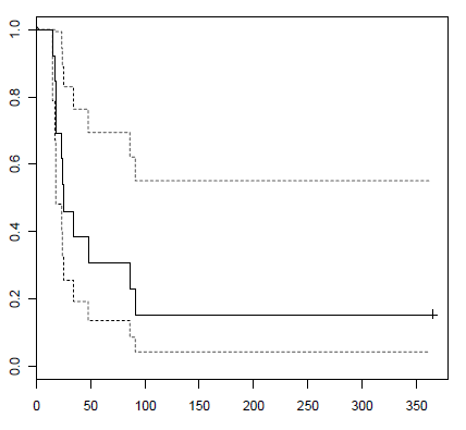
The 'survfit' function from the 'survival' add-on package calculates and plots the Kaplan-Meier survival curve, and also calculates median survival from the Kaplan-Meier curve. The following example analyzes survival for 13 people who were exposed to large doses of radiation during the Chernobyl nuclear accident and received bone marrow transplants (Baranov et.al., NEJM, 1989). The input for the 'survfit( )' function include a variable containing survival/censoring time (days.surv in this example) and an indicator variable for event (coded 1) or censored (coded 0) (death in this example). The 'summary( )' function with survfit gives a listing of the survival function, the 'print( )' function with survfit gives the median survival with a 95% CI, and the 'plot( )' function with survfit gives a plot of the K-M curve with a 95% confidence band (while all 3 functions are illustrated below, it is not necessary to run all three – the K-M plot could be requested directly without printing out the survival proportions).
> summary(survfit(Surv(days.surv,death)))
Call: survfit(formula = Surv(days.surv, death))
time n.risk n.event survival std.err lower 95% CI upper 95% CI
15 13 1 0.923 0.0739 0.7890 1.000
17 12 1 0.846 0.1001 0.6711 1.000
18 11 2 0.692 0.1280 0.4819 0.995
23 9 1 0.615 0.1349 0.4004 0.946
24 8 1 0.538 0.1383 0.3255 0.891
25 7 1 0.462 0.1383 0.2566 0.830
34 6 1 0.385 0.1349 0.1934 0.765
48 5 1 0.308 0.1280 0.1361 0.695
86 4 1 0.231 0.1169 0.0855 0.623
91 3 1 0.154 0.1001 0.0430 0.550
> print(survfit(Surv(days.surv,death)))
Call: survfit(formula = Surv(days.surv, death))
n events median 0.95LCL 0.95UCL
13 11 25 18 Inf
> plot(survfit(Surv(days.surv,death)))
5.2 Kaplan-Meier plots and log-rank test for two groups
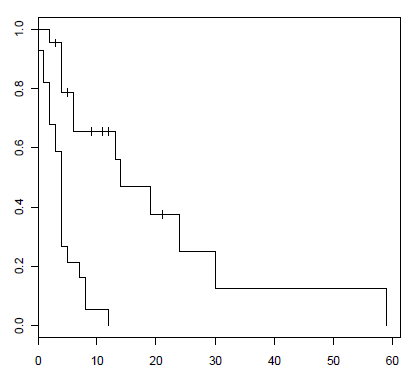
The 'print( )', 'plot( )', and 'survdiff( )' functions in the 'survival' add-ono package can be used to compare median survival times, plot K-M survival curves by group, and perform the log-rank test to compare two groups on survival. In the following example, 'survmonths' is survival time in months, 'event' is an indicator variable coded 1 for those who have had the outcome event and 0 for those who are censored, and 'group' is an indicator variable coded 1 for the experimental and 0 for the control group.
> print(survfit(Surv(survmonths,event) ~ group))
Call: survfit(formula = Surv(survmonths, event) ~ group)
n events median 0.95LCL 0.95UCL
group=0 28 22 4 3 5
group=1 22 12 14 6 Inf
> plot(survfit(Surv(survmonths,event) ~ group))
> survdiff(Surv(survmonths,event) ~ group)
Call:
survdiff(formula = Surv(survmonths, event) ~ group)
N Observed Expected (O-E)^2/E (O-E)^2/V
group=0 28 22 11.3 10.05 20.7
group=1 22 12 22.7 5.02 20.7
Chisq= 20.7 on 1 degrees of freedom, p= 5.33e-06
The chi-square statistic and p-value given above are for the log rank test of the null hypothesis of no difference between the two survival curves.
5.3 Cox's proportional hazards regression for survival data
Cox's proportional hazards regression can be performed using the 'coxph( )' and 'Surv( )' functions of the 'survival' add –on package. R gives the parameter estimates for the Cox model, which can be exponentiated to give estimated hazard ratios (HRs), and confidence intervals for the parameter estimates can be used to get confidence intervals for the hazards ratios. The following performs a proportional hazards regression predicting survival from treatment group (coded 0,1) and age in years, and then finds the HR and 95% CI for the HR comparing groups.
The 'factor( )' function can be used to declare multi-category categorical predictors in a Cox model (to be represented by dummy variables in the model), and the 'relevel(factor( ), ref='') command can be used to specify the reference category in creating dummy variables (see the examples under multiple linear regression and multiple logistic regression above).
> coxph(Surv(survmonths,event) ~ group+age)
Call:
coxph(formula = Surv(survmonths, event) ~ group + age)
coef exp(coef) se(coef) z p
group -1.94034 0.144 0.4872 -3.982 6.8e-05
age 0.00963 1.010 0.0321 0.300 7.6e-01
Likelihood ratio test=20.5 on 2 df, p=3.61e-05 n= 50
> exp(-1.94034)
[1] 0.1436551
> exp(-1.94034-1.93*0.144)
[1] 0.1087983
> exp(-1.94034+1.93*0.144)
[1] 0.1896794
Here, group is significantly related to survival (p<.001), with better survival in the treatment group (group=1) than control group (group=0), with HR=0.143, 95% CI (0.019 , 0.190). Age does not significantly relate to survival (p=0.76).