
Basic Statistical Analysis Using the R Statistical Package
Authors:
Timothy C. Heeren, PhD, Professor of Biostastics
Jacqueline N. Milton, PhD, Clinical Assistant Professor, Biostatistics
Boston University School of Public Health
R is a freely distributed software package for statistical analysis and graphics, developed and managed by the R Development Core Team. R can be downloaded from the Internet site of the Comprehensive R Archive Network (CRAN) (http://cran.r-project.org). Check that you download the correct version of R for your operating system (for example, XP for the PC, Tiger or earlier versions of OSX for Macs). R is related to the S statistical language which is commercially available as S-PLUS.
R is an object-oriented language. For our basic applications, matrices representing data sets (where columns represent different variables and rows represent different subjects) and column vectors representing variables (one value for each subject in a sample) are objects in R. Functions in R perform calculations on objects. For example, if 'cholesterol' was an object representing cholesterol levels from a sample, the function 'mean(cholesterol)' would calculate the mean cholesterol for the sample. For our basic applications, results of an analysis are displayed on the screen. Results from analyses can also be saved as objects in R, allowing the user to manipulate results or use the results in further analyses.
Data can be directly entered into R, but we will usually use MS Excel to create a data set. Data sets are arranged with each column representing a variable, and each row representing a subject; a data set with 5 variables recorded on 50 subjects would be represented in an Excel file with 5 columns and 50 rows. Data can be entered and edited using Excel. Excel can save files in 'comma delimited format', or .csv files; these .csv files can then be read into R for analysis.
R is an interactive language. When you start R, a blank window appears with a '>', which is the ready prompt, on the first line of the window. Analyses are performed through a series of commands; the user enters a command and R responds, the user then enters the next command and R responds. In this document, commands typed in by the user are given in red and responses from R are given in blue; R uses this same color scheme.
Some helpful odds and ends when using R:
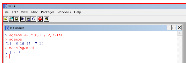
The 'assign operator' in R is used to assign a name to an object. For example, suppose we have a sample of 5 infants with ages (in months) of 6, 10, 12, 7, 15. In R, these values can be represented as a column vector (as a data set, these values would be arranged in one column for the variable age, with 5 rows). To enter these data into R and give the name 'agemos' to these data, we can use the command:
> agemos <- c(6,10,12,7,14)
The '>' is the ready prompt given by R, indicating that R is ready for our input (R typed the >, I typed the rest of the line). Here, agemos is the name we are giving to the object that we will be creating. The '<-' is the assign operator, and the 'c( …)' is a function creating a column vector from the indicated values. So we are creating the object 'agemos' which is a data vector (or variable in a data set).
To print an object, just enter the object name:
> agemos
[1] 6 10 12 7 14
The '[1]' the R gives at the start of the line is a counter – this line starts with the first value in the object (this is helpful with larger data sets when the print out extends over several lines). We can use this object name in later analyses. For example, the mean age of these 5 infants can be calculated using the 'mean( )' function:
> mean(agemos)
[1] 9.8
In R, object names are arbitrary and will generally vary to fit a particular application or study. Functions always involve parentheses to enclose the relevant arguments, and function names make up the R language. So, we might calculate mean age using mean(agemos) or mean cholesterol using mean(cholesterol); the function name is constant, but the object name varies to fit the particular study.
A copy of the R screen for the above analysis, with the input lines that we typed given in red and the output lines that R provides given in blue:
For an analysis of a single variable, with a small number of observations, it is easy to enter a column vector directly into R as described above. But with larger data sets, it is easier to first create and save the data set in Excel, and then to bring information from the Excel file into R. There are several ways to do this. I find it easiest to use the 'read.csv(file.choose))' command, which is described first and uses a Windows-like file menu to find the data file and then bring data into R.
MS Excel is an excellent tool for entering and managing data from a small statistical study. Data are arranged with variables as columns and subjects as rows. The first row of the Excel file (the 'header') can be used to provide variable names (object names for vectors in R). For example, the following are data from the first 5 subjects in a study to compare age first walking between two groups of infants:
|
Subject |
group |
sexmale |
agewalk |
|---|---|---|---|
|
1 |
1 |
1 |
9.00 |
|
2 |
1 |
1 |
9.50 |
|
3 |
1 |
1 |
9.75 |
|
4 |
1 |
0 |
10.00 |
|
5 |
1 |
1 |
13.00 |
Here, "Subject" is an id code; "group" is coded 1 or 2 for the two study groups; "sexmale" is coded 1 for males and 0 for females; and "agewalk" is the age when the infant first walked, in months. Note that I've used single-word (no spaces) variable names; using the underscore '_' or period '.' are nice ways to separate words in a variable name (for example, age_years or age.years are viewed as one-word variable names by R).
To bring an Excel data file into R, it first has to be saved as a comma-delimited file. In Excel, click on 'Save as', and select '.csv' as the file type. Save the file and exit Excel. The .csv file can then be brought into R as a 'data frame' using the 'read.csv(file.choose())' command. Entering
>kidswalk <- read.csv(file.choose())
will open a menu with a file listing for the default directory. See Section 1.3.6 below for instructions on changing the default directory (Link to Changing Default Directory). Double clicking on the data file will bring it into R under the name 'kidswalk'. You can also navigate in the file menu to open .csv files saved in other directories. R will use these object names to identify data, and so the same name cannot be used for both a data frame and a variable name.
The file menu from the 'read.csv(file.choose())' command is illustrated below:
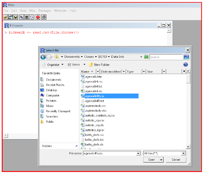
NOTE: Depending on your operating system, R may not be able to read a data file that is opened in another application, and so you may have to close the data set in Excel before being able to read it into R.
NOTE: While the 'read.cvs(file.choose())' function brings a data set into R, there are still some issues with accessing an individual variable from within the data set. Section 1.3.3 below discusses accessing individual variables within a data set.
If you know the name of the file that you want to bring into R, you can read a .csv file directly into R. For example, suppose we saved the data for the Age at Walking example as the file 'agewalk4R.csv' in the R default directory. It can be read in as:
> kidswalk <- read.csv('agewalk4R.csv')
Here, the data set is being saved as a 'data frame' object named 'kidswalk'; the function 'read.csv' reads in the specified .csv file and creates the corresponding R object.
Data sets saved outside the default directory can also be read directly into R, by specifying the folder path (although it may be easier to use the 'file.choose()' command described above). For example:
> kidswalk <- read.csv("C:/Users/tch/Documents/BS703/Data Sets/agewalk4R.csv")
would bring in a data set saved under the BS703/Data Sets folder. Note that forward slashes ( / ) are used in giving the file directory, rather than the backslash ( \ ) used by Windows. R will not recognize paths designated using the usual backslash, and so you must change the slash when cutting-and-pasting directory paths from Windows.
The 'read.csv' command creates an object (dataframe) for the entire data set represented by an Excel file, but it does not create objects for the individual variables. So, while we could perform some analyses on this entire data set, we cannot yet perform analyses on specific variables. When variable names are specified as the first row of the imported Excel file, R creates objects using the 'dataframename$variablename' convention. For example, in the Age First Walking example, after reading in the data set
> kidswalk <- read.csv(file.choose())
the 'agewalk' variable is named 'kidswalk$agewalk', and the 'group' variable is named 'kidswalk$group'. So, to find the mean age at walking, we could enter
> mean(kidswalk$agewalk)
[1] 11.13
For convenience, the individual variables in a data set can also be named without the dataframename prefix. The 'attach()' function creates individual objects for each variable, where the data frame name is specified in the parentheses:
> attach(kidswalk)
This function does not give any visible output, but creates objects (column vectors) for each individual variable in the data set, using the variable names specified in the first row as the object names. For the Age at Walking example, it creates data objects named Subject, group, sexmale, and agewalk. We could then use any of these variable objects in analyses:
> mean(agewalk)
[1] 11.13
Note that R is case-sensitive, and so 'Subject' is a different name than 'subject'. Also, two objects cannot have the same name in R, and so you cannot use the same name for both a dataframe and a variable.
An R dataframe can be viewed and edited as a spreadsheet within R using the R data editor. In R, click on the 'Editor' menu at the top of the R screen, then click on 'Data editor'; this leads to a prompt for the name of the dataframe to view/edit. Or, from the command line, the fix( ) function will open the data editor:
> fix(kidswalk)
The data set appears in a spreadsheet format. Analyses cannot be performed while the data editor is open.
When using Excel to organize data, it is easiest to bring data into R as .csv files. But data may be computerized through other programs, and R can read data saved through other programs as well. The read.table()function reads data that was saved as a text file (with a .txt extension) through MS Word or other programs, with spaces separating the entries in each line of data. As with Excel files, the data set should be set up with columns representing variables and rows representing subjects, and it is helpful to specify variable names as the first row of the document.
> kidswalk <- read.table("agewalk4R.txt")
The same conventions apply to naming individual variables in the data set, as described in 1.3.3 above.
In order to import a saved data set into R, R needs to know which directory (or folder) the data set is saved under on your computer. When you use the 'read.csv(file.choose())' command, you can navigate through folders just as you can with most Windows menus. But you can specify the folder that R first open. The steps for setting the default folder in R differ for PCs and Macs, and instructions for both are given below.
The default folder only needs to be set once, and R will continue to look for files in the default folder.
The default folder for R can be over-written for a single session. After starting R, click on the 'File' menu in the R screen, then select 'Change dir', and specify the directory to be used for this session. R will look for files in this directory for the current session, but will go back to the default directory in future sessions. However, if you 'save the workspace', and the start R by clicking on the saved workspace, settings can be carried over to future sessions.
Many research studies involve some data management before the data are ready for statistical analysis. For example, in using R to manage grades for a course, 'total score' for homework may be calculated by summing scores over 5 homework assignments. Or for a study examining age of a group of patients, we may have recorded age in years but we may want to categorize age for analysis as either under 30 years vs. 30 or more years. R can be used for these data management tasks.
New variables can be calculated using the 'assign' operator. For example, creating a total score by summing 4 scores:
> totscore <- score1+score2+score3+score4
* , / , ^ can be used to multiply, divide, and raise to a power (var^2 will square a variable). As another example, weight in kilograms can be calculated from weight in pounds:
> weight.kg <- 0.4536*weight.lb
The 'ifelse( )' function can be used to create a two-category variable. The following example creates an age group variable that takes on the value 1 for those under 30, and the value 0 for those 30 or over, from an existing 'age' variable:
> ageLT30 <- ifelse(age < 30,1,0)
The arguments for the ifelse( ) command are 1) a conditional expression (here, is age less than 30), then 2) the value taken on if the expression is true, then 3) the value taken on if the expression is false. The expression 'age<=30' would indicate those less than or equal to 30. Logical expressions can be combined as AND or OR with the & and | symbols, respectively. For example, the expression '30 < age & age <=39' would indicate those aged 30 to 39 (age greater than 30 and less than or equal to 39), and 'age<20 | age>70' would indicate those either under 20 or over 70.
In logical expressions, two equal signs are needed for 'is equal to'
(e.g., > obese <- ifelse(BMIgroup==4,1,0), and the 'not equal to' sign in R is '!='.
A series of commands are needed to create a categorical variable that takes on more than two categories. For example, to create an agecat variable that takes on the values 1, 2, 3, or 4 for those under 20, between 20 and 39, between 40 and 59, and over 60, respectively:
> agecat <- 99
> agecat[age<20] <- 1
> agecat[20<=age & age<=39] <- 2
> agecat[40<age & age<=59] <- 3
> agecat[60 <= age] <- 4
The first line creates an 'agecat' variable and assigns each subject a value of 99. The square brackets [ ] (further described in Section 7 below) are used to indicate that an operation is restricted to cases that meet the condition in the brackets. So the 'agecat[age<20] <- 1' statement will assign the value of 1 to the variable agecat, only for those subjects with age less than 20 (over-riding the 99's assigned in the first line of code). The set of four commands assign the values 1 through 4 to the appropriate age groups.
The 'write.csv( )' command can be used to save an R data frame as a .csv file. While variables created in R can be used with existing variables in analyses, the new variables are not automatically associated with a dataframe. For example, suppose we read in a .csv file under the dataframe name 'healthstudy', and that 'age' and 'weight.lb' were variables in this data frame. If we created the 'weight.kg' and 'agecat' variables described above, these variables would be available for analyses in R but would not be part of the 'healthstudy' dataframe. The 'cbind( )' can be used to add new variables to a dataframe (bind new columns to the dataframe). For example,
> healthstudy <- cbind(healthstudy,weight.kg,agecat)
adds the 'weight.kg' variable and the 'agecat' variable to the 'healthstudy' dataframe.
When new variables have been created and added to a dataframe/data set in R, it may be helpful to save this updated data set as a .csv file (which can then be converted to an Excel file or other format). To save a dataframe as a .csv file:
1. First, click on the 'File' menu, click on 'Change directory', and select the folder where you want to save the file.
2. Use the 'write.csv( )' command to save the file:
> write.csv(healthstudy,'healthstudy2.csv')
The first argument (healthstudy) is the name of the dataframe in R, and the second argument in quotes is the name to be given the .csv file saved on your computer. R will overwrite a file if the name is already in use.
The help() function in R provides details for the different R commands. For example,
> help(read.csv)
gives details relating to the read.csv( ) function, while
> help(mean)
gives details for the mean( ) function.
A question mark can also be used to ask for the help function. For example,
> ?read.csv
> ?mean
gives the same help information as the commands above.
The help( ) function only gives information on R functions. To search more broadly, you can use the 'help.search( ) function. For example,
> help.search("t test")
will search for the string 't test' and indicate R functions that reference this string. There is also a fair amount of R help available over the Internet, and googling, for example, 't test R package' may lead to some helpful sites.
The 'mean( )' function calculates means from an object representing either a data matrix or a variable vector. For example, for the 'kidswalk' data set described above, we can calculate the means for all the variables in the data set (a dataframe object):
> mean(kidswalk)
subjno group sex agewalk
25.50 1.34 0.48 11.13
The mean( ) function can also be used to calculate the mean of a single variable (a data vector object):
> mean(agewalk)
[1] 11.13
The 'sd( )' function calculates standard deviations, either for all variables in a data set or for specific variables.
> sd(kidswalk)
subjno group sex agewalk
14.5773797 0.4785181 0.5046720 1.3583078
> sd(agewalk)
[1] 1.358308
The length() function returns the number of values (n, the sample size) in a data vector:
> length(agewalk)
[1] 50
The median of a variable, along with the minimum, maximum, 25th percentile and 75th percentile, are given by the 'summary( )' function:
> summary(Age_walk)
Min. 1st Qu. Median Mean 3rd Qu. Max.
9.00 10.00 11.25 11.13 12.00 13.50
For categorical variables, the 'table( )' function gives the number of subjects in each category, and using the two functions 'prop.table(table( ))' gives the proportion of subjects in each category (although I find it easier to just calculate the proportions from the frequencies). For example, in the age at walking data set, the variable 'sexmale' is coded 0 for females and 1 for males. The number of males and females in the data set are:
> table(sexmale)
sexmale
0 1
26 24
The proportions of males and females can be calculated from the frequencies, using R as a calculator:
> 26/(26+24)
0.52
> 24/(26+24)
0.48
Alternatively, proportions can be calculated using the prop.table( ) command (although this gets a bit complicated in more involved applications):
> prop.table(table(sexmale))
sexmale
0 1
0.52 0.48
There are (at least) three ways to do subgroup analyses in R.
An analysis can be restricted to a subset of subjects using the 'varname[subset]' format. For example,
> mean(agewalk[group==1])
[1] 10.72727
finds the mean of the variable 'agewalk' for those subjects with group equal to 1. When specifying the condition for inclusion in the subset analysis ('Group==1' in this example), two equal signs '==' are needed to indicate a value for inclusion. Less than (<) and greater than (>) arguments can also be used. For example, the following command would find the mean systolic blood pressure for subjects with age over 50:
> mean(sysbp[age>50])
Another approach is to use the tapply() function to perform an analysis on subsets of the data set. The input for the tapply( ) function is 1) the outcome variable (data vector) to be analyzed, 2) the categorical variable (data vector) that defines the subsets of subjects, and 3) the function to be applied to the outcome variable. To find the means, standard deviations, and n's for the two study groups in the 'kidswalk' data set:
> tapply(agewalk, group, mean)
|
1 |
2 |
|
10.72727 |
11.91176 |
> tapply(agewalk, group, sd)
|
1 |
2 |
|
1.231684 |
1.277636 |
> tapply(agewalk, group, length)
1 2
33 17
The subset() function creates a new data frame, restricting observations to those that meet some criteria. For example, the following creates a new data frame for kids in Group 2 of the kidswalk data frame (named 'group2kids'), and finds the n and mean Age_walk for this subgroup:
> group2kids <- subset(kidswalk,Group==2)
> length(group2kids)
[1] 5
> mean(group2kids$Age_walk)
[1] 11.91176
In this example, there are two data sets open in R (kidswalk for the overall sample and group2kids for the subsample) that use the same set of variables names. In this situation, it is helpful to use the 'dataframe$variablename' format to specify a variable name for the appropriate sample.
When specifying the condition for inclusion in the subsample ('Group==2' in this example), two equal signs '==' are needed to indicate a value for inclusion. Less than (<), less than or equal to (<=), greater than (>), greater than or equal to (>=), or not equal to (!=) arguments can also be used. For example,
> age65plus <- subset(allsubjects,age>64)
would create a dataframe of subjects aged 65 and older.
Many research studies involve missing data – not all study variables are measured for on all study subjects. Most functions in R handle missing data appropriately by default, but a couple of basic functions require care when missing data are present. And it's always a good idea to check for missing data in a data set.
When inputting data directly into R, 'NA' is used to designate missing data. For example,
> xvar <- c(2,NA,3,4,5,8)
Creates a variable ('xvar') for a sample of 6 subjects, but the second subject is missing data for this variable. NA is also used to indicate missing data when R prints data:
> xvar
[1] 2 NA 3 4 5 8
When setting up a dataset using Excel, missing data can be represented either by 'NA' or by just leaving the cell blank in Excel. In either case, data will be treated as missing when imported into R.
To check for missing data with a measurement variable, we can use the 'summary( )' command,
> summary(xvar)
Min. 1st Qu. Median Mean 3rd Qu. Max. NA's
2.0 3.0 4.0 4.4 5.0 8.0 1.0
Along with the minimum value, first quartile (25th percentile), median, mean, 3rd quartile and maximum value, the summary command also lists the number of observations with missing data under the NA's column (here there is one subject with missing data). For a categorical variable, we can check for missing data using the 'useNA='always' option in the table( ) command (see sections 15 through 17 for more on the table( ) command):
> table(currsmoke,useNA='always')
currsmoke
0 1 <NA>
11 6 3
In this example of current smoking status, there are 11 non-smokers, 6 smokers, and 3 with missing data.
Most R functions appropriately handle missing data, excluding it from analysis. There are a couple of basic functions where extra care is needed with missing data.
The length( ) command gives the number of observations in a data vector, including missing data. For example, there were 6 subjects in the data set for the 'xvar' variable in the example above, although there were only 5 subjects with actual data and one had a missing value. Using the length( ) function gives
> length(xvar)
[1] 6
which can be misleading, since there are only 5 subjects with valid values for this variable. To find the number of non-missing observations for a variable, we can combine the length( ) function with the na.omit( ) function. The na.omit( ) function omits missing data from a calculation. So, listing the values of xvar gives:
> xvar
[1] 2 NA 3 4 5 8
while listing the non-missing values of xvar gives
> na.omit(xvar)
[1] 2 3 4 5 8
To find the number of non-missing observations for xvar,
> length(na.omit(xvar))
[1] 5
Another common function that does not automatically deal with missing data is the mean( ) function. Trying to calculate a mean for a variable with missing data gives the following:
> mean(xvar)
[1] NA
We can calculate the mean for the non-missing values the 'na.omit( )' function:
> mean(na.omit(xvar))
[1] 4.4
Some functions also have options to deal with missing data. For example, the mean( ) function has the 'na.rm=TRUE' option to remove missing values from the calculation. So another way to calculate the mean of non-missing values for a variable:
> mean(xvar, na.rm=TRUE)
[1] 4.4
See the help( ) function documents in R for options for missing data for specific analyses.
The hist()function draws a histogram of an object representing a variable vector. For a histogram of age of first walking from our example (I copied and pasted the histogram from the R window into this document):
> hist(agewalk)
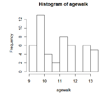
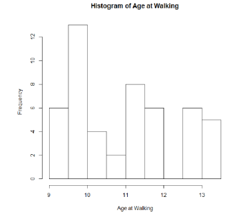
By default, R uses the variable name (agewalk) in the title and x-axis label for the histogram. The default title can be over-written using the 'main=paste( )' option, and the x-axis label can be overwritten using the 'xlab=' option. For example,
> hist(Age_walk,main=paste("Histogram of Age at Walking"),xlab="Age at Walking")
For boxplots comparing the distributions of age of first walking for the two study groups:
> boxplot(agewalk ~ group)
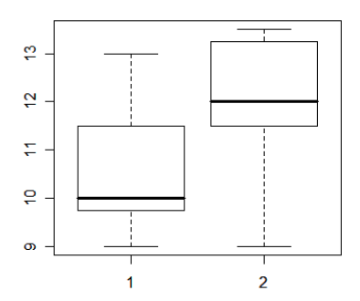
Box plots in R give the minimum, 25th percentile, median, 75th percentile, and maximum of a distribution; observations flagged as outliers (either below Q1-1.5*IQR or above Q3+1.5*IQR) are shown as circles (no observations are flagged as outliers in the above box plot). So, for study group 1, the youngest age at walking was 9 months, the median was about 10 months, and the oldest age at walking was 13 months.
Labels can be added to the x-axis and y-axis using the 'xlab=' and 'ylab=' options:
> boxplot(agewalk ~ group,xlab="Study Group", ylab="Age in Months")
Statistical table functions in R can be used to find p-values for test statistics. See Section 24, User Defined Functions, for an example of creating a function to directly give a two-tailed p-value from a t-statistic.
The pnorm( ) function gives the area, or probability, below a z-value:
> pnorm(1.96)
[1] 0.9750021
To find a two-tailed area (corresponding to a 2-tailed p-value) for a positive z-value:
> 2*(1-pnorm(1.96))
[1] 0.04999579
The qnorm( ) function gives critical z-values corresponding to a given lower-tailed area:
> qnorm(.05)
[1] -1.644854
To find a critical value for a two-tailed 95% confidence interval:
> qnorm(1-.05/2)
[1] 1.959964
The pt( ) function gives the area, or probability, below a t-value. For example, the area below t=2.50 with 25 d.f. is
> pt(2.50,25)
[1] 0.9903284
To find a two-tailed p-value for a positive t-value:
> 2*(1-pt(2.50,25))
[1] 0.01934313
The qt( ) function gives critical t-values corresponding to a given lower-tailed area:
> qt(.05,25)
[1] -1.708141
To find the critical t-value for a 95% confidence interval with 25 degrees freedom:
> qt(1-.05/2,25)
[1] 2.059539
The pchisq( ) function gives the lower tail area for a chi-square value:
> pchisq(3.84,1)
[1] 0.9499565
For the chi-square test, we are usually interested in upper-tail areas as p-values. To find the p-value corresponding to a chi-square value of 4.50 with 1 d.f.:
> 1-pchisq(4.50,1)
[1] 0.03389485
The t.test( ) function performs one-sample and two-sample t-tests. In performing a one-sample t-test, this function also gives a confidence interval for the population mean.
> t.test(agewalk)
One Sample t-test
data: agewalk
t = 57.9405, df = 49, p-value < 2.2e-16
alternative hypothesis: true mean is not equal to 0
95 percent confidence interval:
10.74397 11.51603
sample estimates:
mean of x
11.13
The t.test( ) function can be used to conduct several types of t-tests, and it's a good idea to check the title in the output ('One Sample t-test) and the degrees of freedom (which for a CI for a mean are n-1) to be sure R is performing a one-sample t-test.
If we are interested in a confidence interval for the mean, we can ignore the t-value and p-value given by this procedure (which are discussed in Section 2.2), and focus on the 95% confidence interval. Here, the mean age at walking for the sample of n=50 infants (degrees of freedom are n-1) was 11.13, with a 95% confidence interval of (10.74 , 11.52).
R calculates a 95% confidence interval by default, but we can request other confidence levels using the 'conf.level' option. For example, the following requests the 90% confidence interval for the mean age at walking:
> t.test(agewalk,conf.level=.90)
One Sample t-test
data: agewalk
t = 57.9405, df = 49, p-value < 2.2e-16
alternative hypothesis: true mean is not equal to 0
90 percent confidence interval:
10.80795 11.45205
sample estimates:
mean of x
11.13
Note that R changes the label for the confidence interval (90 percent …) to reflect the specified confidence level.
The prop.test( ) command performs one- and two-sample tests for proportions, and gives a confidence interval for a proportion as part of the output. For example, in the Age at Walking example, 26/50=.52 of the infants were girls. I first used the table() function to find these frequencies, and then calculated the proportion. I then calculated the confidence interval using the prop.test( ) function.
NOTE: When using the prop.test( ) function, specifying 'correct=TRUE' tells R to use the small sample correction when calculating the confidence interval (a slightly different formula), and specifying 'correct=FALSE' tells R to use the usual large sample formula for the confidence interval (Since categorical data are not normally distributed, the usual z-statistic formula for the confidence interval for a proportion is only reliable with large samples - with at least 5 events and 5 non-events in the sample).
> table(sexmale)
sexmale
0 1
26 24
> 26/(26+24)
0.52
> prop.test(26,50,correct=FALSE)
1-sample proportions test without continuity correction
data: 26 out of 50, null probability 0.5
X-squared = 0.02, df = 1, p-value = 0.8875
alternative hypothesis: true p is not equal to 0.5
95 percent confidence interval:
0.3851174 0.6520286
sample estimates:
p
0.52
The prop.test( ) procedure can be used for several scenarios, so it's a good idea to check the labeling (1-sample proportions) to make sure we set things up correctly. The procedure also tests a hypothesis about the proportion (see Section 2.3), but we can focus on the 'p' of 0.52 (the sample proportion) and the confidence interval (0.385 , 0.652). This procedure uses a slightly different formula for the CI than presented in class, and the results of the two versions of the formula may differ slightly. With small samples, it is more appropriate to use the 'correct=TRUE' option to use the correction factor. There is also a 'binom.exact( )' function which calculates a confidence interval for a proportion using an exact formula appropriate for small sample sizes.
The t.test( ) function can also be used to compare means between two samples, and gives the confidence interval for the difference in the means from two independent samples as well as performing the independent samples t-test. For the following syntax, the underlying data set includes the subjects from both samples, with one variable indicating the dependent variable (the outcome variable) and another variable indicating which group a subject is in. The outcome variable and grouping variable are identified using the 'outcome ~ group' syntax. For the usual pooled-variance version of the t-test:
> t.test(agewalk ~ group,var.equal=TRUE)
Two Sample t-test
data: agewalk by group
t = -3.1812, df = 48, p-value = 0.002571
alternative hypothesis: true difference in means is not equal to 0
95 percent confidence interval:
-1.9331253 -0.4358587
sample estimates:
mean in group 1 mean in group 2
10.72727 11.91176
The t.test( ) function can be used to conduct several types of t-tests, with several different data set ups, and it's a good idea to check the title in the output ('Two Sample t-test) and the degrees of freedom (n1 + n2 – 2) to be sure R is performing the pooled-variance version of the two sample t-test.
The t-statistic and p-value are discussed under Section 2.2.2. The 95% confidence interval that is given is for the difference in the means for the two groups (10.73 – 11.91 gives a difference in means of -1.18, and the CI that R gives is a CI for this difference in means). By default, R gives the 95% CI; the 'conf.level' level option can be used to change the confidence level (see Section 2.1.1). Note that the output gives the means for each of the two groups being compared, but not the standard deviations or sample sizes. This additional information can be obtained using the tapply( ) function as described in Section 7 (in this example, tapply(agewalk,group,sd) will give standard deviations, table(group) will give n's).
To calculate the confidence interval for the difference in means using the unequal variance formula:
> t.test(agewalk ~ group,var.equal=FALSE)
Welch Two Sample t-test
data: agewalk by group
t = -3.1434, df = 31.39, p-value = 0.003635
alternative hypothesis: true difference in means is not equal to 0
95 percent confidence interval:
-1.9526304 -0.4163536
sample estimates:
mean in group 1 mean in group 2
10.72727 11.91176
Again, it's good to check the title (Welch Two Sample t-test) and degrees of freedom (which often take on decimal values for the unequal variance version of the t-test) to be sure R is using the unequal variance formula for the confidence interval and t-test.
The t.test( ) function can also be used to calculate the confidence interval for a mean from a paired (pre-post) sample, and to perform the paired-sample t-test. In this situation, we need to specify the two data vectors representing the two variables to be compared. The following example compares the means of a pre-test score (score1) and a post-test score (score2) from a sample of 5 subjects. The t.test( ) function does not give the means of the two underlying variables (it does give the mean difference) and so I used the mean( ) function to get this descriptive information. Generally standard deviations and sample size would also be reported, which can be obtained from the sd( ) and length( ) functions.
> mean(score1)
[1] 20.2
> mean(score2)
[1] 21
> t.test(score1,score2,paired=TRUE)
Paired t-test
data: score1 and score2
t = -0.4377, df = 4, p-value = 0.6842
alternative hypothesis: true difference in means is not equal to 0
95 percent confidence interval:
-5.874139 4.274139
sample estimates:
mean of the differences
-0.8
The t.test( ) function can be used for several different types of t-tests, and so it's a good idea to check the title (Paired t-test) and degrees of freedom (n-1, where n is the number of pairs in the study) to be sure R is performing a paired sample analysis.
The confidence interval here is the confidence interval for the mean difference; the confidence interval should agree with the p-value in that the CI should not contain 0 when p<0.05, and the CI should contain 0 when p>0.05.
Note that the t.test( ) procedure gives the mean difference, but does not give the standard deviations of the difference or the standard deviations of the two variables. Generally, standard deviations are reported as part of the data summary for a comparison of means, and these standard deviations can be found using the 'sd( )' command.
The prop.test( ) command performs a two-sample test for proportions, and gives a confidence interval for the difference in proportions as part of the output. The example below uses data from the Age at Walking example, comparing the proportion of infants walking by 1 year in the exercise group (group=1) and control group (group=2). The table( ) command is used to find the number of infants walking by 1 year in each study group, and the proportion walking can be calculated from these frequencies. The prop.test( ) command will calculate a confidence interval for the difference between two proportions; for the two-sample situation, first enter a vector representing the number of successes in each of the two groups (using the c( ) command to create a column vector), and then a vector representing the number of subjects in each of the two groups. To use the usual large-sample formula in calculating the confidence interval, include the 'correct=FALSE' option to turn off the small sample size correction factor in the calculation (although in this example, with only 17 subjects in the control group, the small sample version of the confidence interval might be more appropriate).
> table(by1year,group)
group
by1year 1 2
0 5 9
1 28 8
> 28/33
0.848
> 8/17
0.470
> prop.test(c(28,8),c(33,17),correct=FALSE)
2-sample test for equality of proportions without continuity
correction
data: c(28, 8) out of c(33, 17)
X-squared = 7.9478, df = 1, p-value = 0.004815
alternative hypothesis: two.sided
95 percent confidence interval:
0.1109476 0.6448456
sample estimates:
prop 1 prop 2
0.8484848 0.4705882
Warning message:
In prop.test(c(28, 8), c(33, 17), correct = FALSE) :
Chi-squared approximation may be incorrect
The prop.test( ) command does several different analyses, and it's a good idea to check the title to make sure R is comparing two groups ('2-sample test for equality…'). The procedure also gives the results of a chi-square test comparing the two proportions (see Section 2.5), but here we are interested in the confidence interval and the proportions in each study group. For this example, 84.8% of the exercise group was walking by 1 year, and 47.1% of the control group was walking by 1 year. The difference in these two proportions is 84.8 – 47.1 = 37.7, and the 95% CI for this difference is (11.1% , 64.5%). We are 95% confident that more infants walk by 1 year in the exercise group (since this interval does not contain 0); we are 95% confident that the additional percent of kids walking by 1 year is between 11.1% and 64.5%.
Epidemiologic analyses are available through 'epitools', an add-on package to R. To use the epitools functions, you must first do a one-time installation. In R, click on the 'Packages' menu, then 'Install Package(s)', then select a download site (from the US), then select the epitools package. This will install the add-on package onto your computer. To use the package, you must also load it into R: click on the 'Packages' menu, then 'Load Package', then select epitools. While you only need to install the package once onto your computer, you will need to load the package into R each time you want to use it.
The data layout matters for calculating RRs. For the riskratio( ) function from epitools, data should be set up in the following format:
|
|
No Disease |
Disease |
|---|---|---|
|
Control |
|
|
|
Exposed |
|
|
This data layout corresponds to the usual 0/1 coding for the exposure and disease variables, but is slightly different than the layout traditionally used in the Introductory Epidemiology class (so be careful!). The riskratio( ) command calculates the RR of disease for those in the exposed group relative to the control group.
Using the Age at Walking example, I'll find the relative risk of being a late walker (walking at 12 months or older) for those in the non-exercise group compared to those in the exercise group. I first created two 0/1 dichotomous variables (see Section 1.4.2 on creating new variables) to reflect the RR of interest: NoExercise is coded 1 for those in the non-exercise control group and 0 for those in the exercise group; LateWalker is coded 1 for those walking at 12 months or later and 0 for those walking before 12 months. With the variables defined in this manner, the table should be oriented correctly for the RR of interest. I first printed the 2x2 table as a check, then used the riskratio() function to calculate the relative risk and large sample 95% confidence interval.
> table(NoExercise,LateWalker)
LateWalker
NoExercise 0 1
0 28 5
1 8 9
> riskratio.wald(NoExercise,LateWalker)
$data
Outcome
Predictor 0 1 Total
0 28 5 33
1 8 9 17
Total 36 14 50
$measure
risk ratio with 95% C.I.
Predictor estimate lower upper
0 1.000000 NA NA
1 3.494118 1.387688 8.797984
$p.value
two-sided
Predictor midp.exact fisher.exact chi.square
0 NA NA NA
1 0.008000253 0.007949207 0.004814519
$correction
[1] FALSE
attr(,"method")
[1] "Unconditional MLE & normal approximation (Wald) CI"
Warning message:
In chisq.test(xx, correct = correction) :
Chi-squared approximation may be incorrect
The RR here is 3.49 ( (9/17) / (5/33) ) , with a 95% CI of (1.39 , 8.80). There are several versions of a CI for a relative risk, and using 'riskratio.wald( )' requests the standard normal approximation formula; 'riskratio.small( )' uses a correction to the CI for small samples (and the 'Warning message' that R gave in the above example, that the 'Chi-squared approximation may be incorrect' is a small sample size warning). R will choose the appropriate version of the CI if 'riskratio( )' is specified.
Cell counts from a 2x2 table (or larger tables) can also be entered directly into R for analysis (RR, OR, or chi-square analysis). For example, the following table presents data on adverse side effects for patients undergoing robot-assisted vs. traditional surgery:
|
|
No Side Effect |
Side Effect |
Total |
|---|---|---|---|
|
Traditional |
5169 |
111 |
5280 |
|
Robo-Assist |
3355 |
165 |
3520 |
The rate of side effects was 2.1% (111/5280) vs. 4.7% (165/3520) for those undergoing traditional vs. robot-assisted surgery. Table orientation matters for the RR (see Section 2.1.6.1), and this table is set up to find the RR of a side effect, for those undergoing robot-assisted compared to traditional surgery.
The matrix(c( ),nrow=,ncol= ) command can be used to enter cell counts from a table directly into R. R treats data entered using the column command (c( ) ) as columns of numbers, so data must be entered by column – counts for the first column followed by counts for the second column. The 'nrow=' and 'ncol=' command specify the dimensions of the table (here, 2 rows and 2 columns). The following commands enter and save the above table as 'sideeffects', prints the table as a check to be sure the table is oriented correctly, and then finds the RR and 95% CI:
> sideeffects <- matrix(c(5169,3355,111,165),nrow=2,ncol=2)
> sideeffects
[,1] [,2]
[1,] 5169 111
[2,] 3355 165
> riskratio.wald(sideeffects)
$data
Outcome
Predictor Disease1 Disease2 Total
Exposed1 5169 111 5280
Exposed2 3355 165 3520
Total 8524 276 8800
$measure
risk ratio with 95% C.I.
Predictor estimate lower upper
Exposed1 1.00000 NA NA
Exposed2 2.22973 1.759603 2.825463
$p.value
two-sided
Predictor midp.exact fisher.exact chi.square
Exposed1 NA NA NA
Exposed2 1.857736e-11 2.056211e-11 9.338045e-12
$correction
[1] FALSE
attr(,"method")
[1] "Unconditional MLE & normal approximation (Wald) CI"
Those given robot-assisted surgery had 2.23 times the odds of an adverse side effect, compared to those given traditional surgery; we are 95% confident that the true RR is between 1.76 and 2.83.
The epitools add-on package also has a function to calculate odds ratios and confidence intervals for odds ratios. You must first load the epitools package into R (see Section 2.1.6). Orientation of the table matters when calculating the OR, and the orientation described above for the relative risk also applies for the odds ratio. The oddsratio.wald( ) command can be used with a per-subject data set or can be used to find the OR and CI from summarized cell counts entered directly into R (see the matrix( ) command described in Section 2.1.6.2).
Calculating the odds ratio ( (9/8) / (5/28) = 6.3 ) and 95% CI for late walkers (see the example in 2.1.6 above), for non-exercisers vs. exercisers in the Age at Walking example:
> oddsratio.wald(NoExercise,LateWalker)
$data
Outcome
Predictor 0 1 Total
0 28 5 33
1 8 9 17
Total 36 14 50
$measure
odds ratio with 95% C.I.
Predictor estimate lower upper
0 1.0 NA NA
1 6.3 1.639283 24.2118
$p.value
two-sided
Predictor midp.exact fisher.exact chi.square
0 NA NA NA
1 0.008000253 0.007949207 0.004814519
$correction
[1] FALSE
attr(,"method")
[1] "Unconditional MLE & normal approximation (Wald) CI"
Warning message:
In chisq.test(xx, correct = correction) :
Chi-squared approximation may be incorrect
The 'oddsratio.wald" option gives the usual estimate for the odds ratio, with OR=6.3 and 95% CI of 1.64 , 24.21. 'oddsratio.small( )' uses a correction for small sample size in calculating the CI.
The one-sample t-test compares the mean from one sample to some hypothesized value. The t.test( ) function performs a one-sample t-test. For input, we need to specify the variable (vector) that we want to test, and the hypothesized mean value. To test whether the mean age at walking is equal to 12 months for the infants in our age of first walking example:
> t.test(agewalk,mu=12)
One Sample t-test
data: agewalk
t = -4.529, df = 49, p-value = 3.806e-05
alternative hypothesis: true mean is not equal to 12
95 percent confidence interval:
10.74397 11.51603
sample estimates:
mean of x
11.13
The t.test()function can be used to conduct several types of t-tests, and it's a good idea to check the title in the output ('One Sample t-test) and the degrees of freedom (n-1 for a one-sample t-test) to be sure R is performing a one-sample t-test.
R performs a two-tailed test, as indicated by the two-tailed language in the alternative hypothesis. The p-value here is given in scientific notation, and the 'e-05' indicates that the decimal place should be moved 5 spaces to the left; 3.806e-05 is scientific notation for 0.00003806, which would generally be reported as 'p<.001'. R also gives the 95% confidence interval for the mean; if there is no significant difference between the sample mean and the hypothesized value (i.e., if the p-value is greater than .05), the confidence interval for the mean will contain the hypothesized value. If there is a significant difference between the sample mean and the hypothesized mean, the confidence interval will not contain the hypothesized value.
Note that the t.test( ) function does give the mean, but does not give the standard deviation or sample size which are usually reported along with a mean (although, for a one sample test, sample size can be determined from the degrees freedom which are given). This information can be obtained using the sd( ) function and the length( ) function (sd(agewalk) and length(agewalk) for this example – although care is needed with the length( ) command when there are missing values.
The t.test( ) function can also be used to perform an independent samples t-test comparing means from two independent samples. For the following syntax, the underlying data set includes the subjects from both samples, with one variable indicating the dependent variable (the outcome variable) and another variable indicating which group a subject is in. To perform the independent samples t-test, we need to specify the object representing the dependent variable and the object representing the group information. For the usual pooled-variance version of the t-test:
> t.test(agewalk ~ group,var.equal=TRUE)
Two Sample t-test
data: agewalk by group
t = -3.1812, df = 48, p-value = 0.002571
alternative hypothesis: true difference in means is not equal to 0
95 percent confidence interval:
-1.9331253 -0.4358587
sample estimates:
mean in group 1 mean in group 2
10.72727 11.91176
The t.test( ) function can be used to conduct several types of t-tests, with several different data set ups, and it's a good idea to check the title in the output ('Two Sample t-test) and the degrees of freedom (n1 + n2 – 2) to be sure R is performing the pooled-variance version of the two sample t-test.
R reports a two-tailed p-value, as indicated by the two-tailed phrasing of the alternative hypothesis. The 95% confidence interval that is given is for the difference in the means for the two groups (10.73 – 11.91 gives a difference in means of -1.18, and the CI that R gives is a CI for this difference in means). Note that the output gives the means for each of the two groups being compared, but not the standard deviations or sample sizes. This additional information can be obtained using the tapply( ) function as described in Section 7 (in this example, tapply(agewalk,group,sd) will give standard deviations, table(group) will give n's).
To perform an independent sample t-test using the unequal variance version of the t-test:
> t.test(agewalk ~ group,var.equal=FALSE)
Welch Two Sample t-test
data: agewalk by group
t = -3.1434, df = 31.39, p-value = 0.003635
alternative hypothesis: true difference in means is not equal to 0
95 percent confidence interval:
-1.9526304 -0.4163536
sample estimates:
mean in group 1 mean in group 2
10.72727 11.91176
Again, it's good to check the title (Welch Two Sample t-test) and degrees of freedom (which often take on decimal values for the unequal variance version of the t-test) to be sure R is performing the unequal variance version of the two sample t-test. As discussed above, standard deviations and sample sizes are also usually given as part of the summary for a two-sample t-test.
The t.test( ) function can also be used to perform a paired-sample t-test. In this situation, we need to specify the two data vectors representing the two variables to be compared. The following example compares the means of a pre-test score (variable score1) and a post-test score (variable score2) from a sample of 5 subjects. The t.test( ) function does not give the means of the two underlying variables (it does give the mean difference) and so I used the mean( ) function to get this descriptive information. Generally standard deviations and sample size would also be reported, which can be obtained from the sd( ) and length( ) functions.
> mean(score1)
[1] 20.2
> mean(score2)
[1] 21
> t.test(score1,score2,paired=TRUE)
Paired t-test
data: score1 and score2
t = -0.4377, df = 4, p-value = 0.6842
alternative hypothesis: true difference in means is not equal to 0
95 percent confidence interval:
-5.874139 4.274139
sample estimates:
mean of the differences
-0.8
The t.test( ) function can be used for several different types of t-tests, and so it's a good idea to check the title (Paired t-test) and degrees of freedom (n-1, where n is the number of pairs in the study) to be sure R is performing a paired sample test.
The confidence interval here is the confidence interval for the mean difference; the confidence interval should agree with the p-value in that the CI should not contain 0 when p<0.05, and the CI should contain 0 when p>0.05.
Note that the t.test( ) procedure gives the mean difference, but does not give the standard deviations of the difference or the standard deviations of the two variables. Generally, standard deviations are reported as part of the data summary for a comparison of means, and these standard deviations can be found using the 'sd( )' command.
The prop.test( ) command performs one- and two-sample tests for proportions, and gives a confidence interval for a proportion as part of the output. For example, in the Age at Walking example, let's test the null hypothesis that 50% of infants start walking by 12 months of age. By default, R will perform a two-tailed test. The variable 'walkby12' that takes on the value of 1 for infants who walked by 1 year of age, and 0 for infants who did not start walking until after they were a year old. Using the table( ) command shows that, in this sample, 36/50=.72 of the infants walked by 1 year. The prop.test( ) procedure will perform the z-test comparing this proportion to the hypothesized value; input for the prop.test is the number of events (36), the total sample size (50), the hypothesized value of the proportion under the null (p=0.50 for a null value of 50%). Specifying 'correct=TRUE' tells R to use the small sample correction when calculating the confidence interval (a slightly different formula), and specifying 'correct=FALSE' tells R to use the usual large sample formula for the z-test for a proportion (since categorical data are not normally distributed, the usual z-statistic formula for the confidence interval for a proportion is only reliable with large samples - with at least 5 events and 5 non-events in the sample).
> table(walkby12)
walkby12
0 1
14 36
> prop.test(36,50,p=0.5,correct=FALSE)
1-sample proportions test without continuity correction
data: 36 out of 50, null probability 0.5
X-squared = 9.68, df = 1, p-value = 0.001863
alternative hypothesis: true p is not equal to 0.5
95 percent confidence interval:
0.5833488 0.8252583
sample estimates:
p
0.72
The prop.test( ) procedure can be used for several scenarios, so it's a good idea to check the labeling (1-sample proportions) to make sure we set things up correctly. 72% of infants began walking before age 12 months. The two-tailed p-value here is p=0.0018, which is less than the conventional cut-off of 0.05, and so we can conclude that the percent of infants walking before age 12 months is significantly greater than 50%. The prop.test( ) procedure also gives a confidence interval for this proportion tests a hypothesis about the proportion (see Section 2.1.2). Note that the CI here does not contain the null value of 0.50, agreeing with the p-value that the percent walking by age 12 is greater than 50%.
There is also a 'binom.exact( )' function which calculates a confidence interval for a proportion using an exact formula appropriate for small sample sizes.
The prop.test( ) command performs a two-sample test for proportions, and gives a confidence interval for the difference in proportions as part of the output. The z-test comparing two proportions is equivalent to the chi-square test of independence, and the prop.test( ) procedure formally calculates the chi-square test. The p-value from the z-test for two proportions is equal to the p-value from the chi-square test, and the z-statistic is equal to the square root of the chi-square statistic in this situation.
The example below uses data from the Age at Walking example, comparing the proportion of infants walking by 1 year in the exercise group (group=1) and control group (group=2). The table( ) command is used to find the number of infants walking by 1 year in each study group, and the proportion walking can be calculated from these frequencies. The prop.test( ) command performs the chi-square test comparing the two proportions; for the two-sample situation, first enter a vector representing the number of successes in each of the two groups (using the c( ) command to create a column vector), and then a vector representing the number of subjects in each of the two groups. To use the usual large-sample formula in calculating the confidence interval, include the 'correct=FALSE' option to turn off the small sample size correction factor in the calculation (although in this example, with only 17 subjects in the control group, the small sample version of the confidence interval might be more appropriate).
> table(by1year,group)
group
by1year 1 2
0 5 9
1 28 8
> 28/33
0.848
> 8/17
0.470
> prop.test(c(28,8),c(33,17),correct=FALSE)
2-sample test for equality of proportions without continuity
correction
data: c(28, 8) out of c(33, 17)
X-squared = 7.9478, df = 1, p-value = 0.004815
alternative hypothesis: two.sided
95 percent confidence interval:
0.1109476 0.6448456
sample estimates:
prop 1 prop 2
0.8484848 0.4705882
Warning message:
In prop.test(c(28, 8), c(33, 17), correct = FALSE) :
Chi-squared approximation may be incorrect
The prop.test( ) command does several different analyses, and it's a good idea to check the title to make sure R is comparing two groups ('2-sample test for equality…'). The p-value (p=0.0048) is a two-tailed p-value testing the null hypothesis of no difference between the two proportions. Since the p-value is less than the conventional 0.05, this example shows a significant difference in the percent of infants walking by 1 year; more infants in the exercise group are walking by 1 year than in the control group. The procedure gives a chi-square statistic which is equal to the square of the z-statistic. Here the z-statistic would be the square root of 7.9478 or z=2.819. The procedure also gives the results of a confidence interval for the difference between the two proportions (see section 2.1.5).
As an example, suppose we want to compare the mean days to healing for 5 different treatments for fever blisters.
The data set includes four variables:
When R performs an ANOVA, there is a lot of potential output. So I generally save the 'results' of the ANOVA as an object, and then ask for different parts of the output through different commands. To perform the ANOVA:
> fever_anova <- aov(DaysHeal ~ TreatName)
Here I've saved the results of the ANOVA as an object named 'fever_anova':
(If the grouping variable is a numeric variable, you can declare it to be categorical using the factor( ) function. For example, for the numeric 'Treatment' variable, the above ANOVA command becomes
> fever_anova <- aov(DaysHeal ~ factor(Treatment) )
This gives the same results as the above analysis.)
We can now request different summary results about the analysis using the results of this analysis. To see the means for the study groups:
> model.tables(fever_anova,"means",digits=3)
Tables of means
Grand mean
5.633333
TreatmentF
TreatmentF
1 2 3 4 5
7.500 5.000 4.333 5.167 6.167
The select if command or the tapply( ) function can be used to get standard deviations and sample sizes for each group, as described in Section 5b: Finding means and standard deviations for subgroups.
To request the ANOVA table and p-value for the overall ANOVA comparing means across the 5 groups:
> summary(fever_anova)
Df Sum Sq Mean Sq F value r(>F)
TreatmentF 4 36.467 9.117 3.896 0.01359 *
Residuals 25 58.500 2.340
---
Signif. codes: 0 '***' 0.001 '**' 0.01 '*' 0.05 '.' 0.1 ' ' 1
Given the overall ANOVA shows significance, we can request pairwise comparisons using Tukey's multiple comparison procedure:
> TukeyHSD(fever_anova)
Tukey multiple comparisons of means
95% family-wise confidence level
Fit: aov(formula = DaysHeal ~ TreatmentF)
$TreatmentF
diff lwr upr p adj
2-1 -2.5000000 -5.0937744 0.09377442 0.0627671
3-1 -3.1666667 -5.7604411 -0.57289224 0.0113209
4-1 -2.3333333 -4.9271078 0.26044109 0.0927171
5-1 -1.3333333 -3.9271078 1.26044109 0.5660002
3-2 -0.6666667 -3.2604411 1.92710776 0.9410027
4-2 0.1666667 -2.4271078 2.76044109 0.9996956
5-2 1.1666667 -1.4271078 3.76044109 0.6811222
4-3 0.8333333 -1.7604411 3.42710776 0.8770466
5-3 1.8333333 -0.7604411 4.42710776 0.2614661
5-4 1.0000000 -1.5937744 3.59377442 0.7881333
The following gives the syntax needed to calculate a chi-square goodness-of-fit test from a set of tabled frequencies. As an example, 45 subjects are asked which of 3 screening tests they prefer; 10 subjects prefer Test A, 15 prefer test B, and 20 prefer Test C. We wish to test the null hypothesis that the three screening tests are equally preferred, or equivalently, that 1/3 of subjects prefer each test. The data:
|
Preference |
Observed Frequency |
Expected Proportion Under the Null |
|---|---|---|
|
Test A |
10 |
0.333 |
|
Test B |
15 |
0.333 |
|
Test C |
20 |
0.333 |
To analyze these data in R, first create an object (arbitrarily named 'obsfreq' in the example) that contains the observed frequencies. Second, we create an object that contains the expected probabilities under the null (arbitrarily named 'nullprobs'; the third probability was rounded to .334 because the probabilities must sum to 1.00; perhaps a better solution would have been to give the probabilities as 1/3,1/3,1/3, which would also work). Third, we compare the observed frequencies to the expected probabilities through the chisq.test( ) function:
> obsfreq <- c(10,15,20)
> nullprobs <- c(.333,.333,.334)
> chisq.test(obsfreq,p=nullprobs)
Chi-squared test for given probabilities
data: x
X-squared = 3.3018, df = 2, p-value = 0.1919
R gives a two-tailed p-value.
From the Age at Walking example, suppose we want to compare the percent of males (coded sexmale=1) between the two groups in our age first walking example. We can first use the 'table( )' function to get the observed counts for the underlying frequency table:
> table(group,sexmale)
sexmale
group 0 1
1 17 16
2 9 8
In group 1, there are 16 males and 17 females, so 48.5% (16/33) of group 1 is male.
In group 2, 47.1% (8/17) are male. The 'prop.table( )' function will calculate these proportions in R:
> prop.table(table(group,sexmale),1)
sexmale
group 0 1
1 0.5151515 0.4848485
2 0.5294118 0.4705882
The 'prop.table( )' command calculates proportions from the indicated table; in this example we want to calculate proportions within groups, and the '1' in the 'prop.table( )' example above indicates that we want proportions calculated within groups for the first variable in the table (within group, so we're calculating the percent of males and females within group 1, and the percent of males and females within group 2). Had we indicated '2' in the above example, R would have calculated proportions within sex, giving the proportions in groups 1 and 2 for males, and the proportions within groups 1 and 2 for females.
Specifying the orientation for the prop.table( ) command can be confusing, and it may be easier (or safer) to just calculate proportions directly for the table of counts. R can be used as a calculator to find these proportions directly:
> 16/(16+17)
[1] 0.4848485
> 8/(8+9)
[1] 0.4705882
The chisq.test() function applied to a table object compares these two percentages through the chi-square test of independence:
> chisq.test(table(group,sexmale),correct=FALSE)
Pearson's Chi-squared test
data: table(group, sexmale)
X-squared = 0.0091, df = 1, p-value = 0.9238
The 'correct=FALSE' option in the chisq.test function turns off Yates' correction for the chi-square test (which is used with small sample sizes), and gives the standard chi-square test statistic. R gives a two-tailed p-value. Note that the title for the output, 'Pearson's Chi-squared test' indicates that these results are for the uncorrected (not Yates' adjusted) chi-square test.
R can also perform a chi-square test on frequencies from a contingency table. For example, suppose we want to compare percent of subjects testing positive on a marker for an exposure across three groups:
|
|
Group 1 |
Group 2 |
Group 3 |
|---|---|---|---|
|
Test Positive |
20 (40%) |
5 (33.3% |
40 (50%0 |
|
Test Negative |
30 |
10 |
40 |
First, we create an object ('obsfreq' in the example) containing the observed frequencies from the observed table. I printed the object as a check that it was created correctly:
> obsfreq <- matrix(c(20,30, 5,10, 40,40),nrow=2,ncol=3)
> obsfreq
[,1] [,2] [,3]
[1,] 20 5 40
[2,] 30 10 40
The 'chisq.test( )' function will then calculate the chi-square statistic for the test of independence for this table:
> chisq.test(obsfreq)
Pearson's Chi-squared test
data: obsfreq
X-squared = 2.1378, df = 2, p-value = 0.3434
The usual chi-square test is appropriate for large sample sizes. For 2x2 tables with small samples (an expected frequency less than 5), the usual chi-square test exaggerates significance, and Fisher's exact test is generally considered to be a more appropriate procedure. The fisher.test() function performs Fisher's exact test in R:
> fisher.test(group,sexmale)
Fisher's Exact Test for Count Data
data: group and sexmale
p-value = 1
alternative hypothesis: true odds ratio is not equal to 1
95 percent confidence interval:
0.2480199 3.5592990
sample estimates:
odds ratio
0.9455544
R gives the two-tailed p-value, as indicated by the wording of the alternative hypothesis. The odds ratio and a 95% confidence interval for the odds ratio are also given. Since Fisher's test is usually used for small sample situations, the CI for the odds ratio includes a correction for small sample sizes.
Epidemiologic analyses are available through 'epitools', an add-on package to R. To use the epitools functions, you must first do a one-time installation. In R, click on the 'Packages' menu, then 'Install Package(s)', then select a download site (from the US), then select the epitools package. This will install the add-on package onto your computer. To use the package, you must also load it into R: click on the 'Packages' menu, then 'Load Package', then select epitools. While you only need to install the package once onto your computer, you will need to load the package into R each time you want to use it.
The data layout matters for calculating RRs. For the riskratio( ) function from epitools, data should be set up in the following format:
|
|
No Disease |
Disease |
|---|---|---|
|
Control |
|
|
|
Exposed |
|
|
riskratio( ) calculates the RR of disease for those in the exposed group relative to the control group.
For the Age at Walking example, I categorized age at walking as early walking (under 12 months, coded 0) and late walking (12 months or older, coded 1). To find the relative risk for late walking, for kids in Group 2 vs. Group 1, I first printed the 2x2 table as a check, then used the riskratio() function to calculate the relative risk and large sample 95% confidence interval.
> table(group,LateWalker)
LateWalker
group FALSE TRUE
1 28 5
2 8 9
> riskratio.wald(group,LateWalker)
$data
Outcome
Predictor FALSE TRUE Total
1 28 5 33
2 8 9 17
Total 36 14 50
$measure
risk ratio with 95% C.I.
Predictor estimate lower upper
1 1.000000 NA NA
2 3.494118 1.387688 8.797984
$p.value
two-sided
Predictor midp.exact fisher.exact chi.square
1 NA NA NA
2 0.008000253 0.007949207 0.004814519
$correction
[1] FALSE
attr(,"method")
[1] "Unconditional MLE & normal approximation (Wald) CI"
Warning message:
In chisq.test(xx, correct = correction) :
Chi-squared approximation may be incorrect
The RR here is 3.49 ( (9/17) / (5/33) ) , with a 95% CI of (1.39 , 8.80). There are several versions of a CI for a relative risk, and using 'riskratio.wald( )' requests the standard normal approximation formula; 'riskratio.small( )' uses a correction to the CI for small samples. R will choose the appropriate version of the CI if 'riskratio( )' is specified.
The epitools add-on package also has a function to calculate odds ratios and confidence intervals for odds ratios. You must first load the epitools package into R (see Section 16d). Orientation of the table matters when calculating the OR, and the orientation described above for the relative risk also applies for the odds ratio. Calculating the odds ratio ( (9/8) / (5/28) = 6.3 ) and 95% CI for late walkers, for Group 2 vs. Group 1 in the Age at Walking example:
> oddsratio.wald(group,LateWalker)
$data
Outcome
Predictor FALSE TRUE Total
1 28 5 33
2 8 9 17
Total 36 14 50
$measure
odds ratio with 95% C.I.
Predictor estimate lower upper
1 1.0 NA NA
2 6.3 1.639283 24.2118
$p.value
two-sided
Predictor midp.exact fisher.exact chi.square
1 NA NA NA
2 0.008000253 0.007949207 0.004814519
$correction
[1] FALSE
attr(,"method")
[1] "Unconditional MLE & normal approximation (Wald) CI"
Warning message:
In chisq.test(xx, correct = correction) :
Chi-squared approximation may be incorrect
The 'oddsratio.wald" option gives the usual estimate for the odds ratio, with OR=6.3 and 95% CI of 1.64 , 24.21. 'oddsratio.small( )' uses a correction for small sample size in calculating the CI.
The wilcox.test( ) function performs the Wilcoxon rank sum test (for two independent samples, with the 'paired=FALSE option) and the Wilcoxon signed rank test (for paired samples, with the 'paired=TRUE' option). With samples less than 50 and no ties, R calculates an exact p-value, otherwise R uses a normal approximation with a correction factor to calculate a p-value.
To perform a Wilcoxon rank sum test, data from the two independent groups must be represented by two data vectors. In this example, we want to compare lactate levels for subjects from Group=1 vs. Group=2 (the original data frame contains data on subjects from both study groups, with the Group variable indicating group membership). The following commands create separate data vectors for lactate for subjects in the two study groups (see Section 7 for the subset command; I printed the two data vectors as a check):
> lactate.sga <- subset(Lactate,Group==2)
> lactate.controls <- subset(Lactate,Group==1)
> lactate.sga
[1] 5.79 4.60 4.20 1.65 2.38 5.67 12.60 3.40 7.57 2.48 4.36
> lactate.controls
[1] 3.18 2.52 1.40 2.26 1.61
The following performs the Wilcoxon rank sum test. Note that the wilcox.test function does not provide any descriptive statistics, and so the summary( ) function was used to find medians and interquartile ranges for the two groups.
> wilcox.test(lactate.sga,lactate.controls,paired=FALSE)
Wilcoxon rank sum test
data: lactate.sga and lactate.controls
W = 48, p-value = 0.01923
alternative hypothesis: true location shift is not equal to 0
> summary(lactate.sga)
Min. 1st Qu. Median Mean 3rd Qu. Max.
1.650 2.940 4.360 4.973 5.730 12.600
> summary(lactate.controls)
Min. 1st Qu. Median Mean 3rd Qu. Max.
1.400 1.610 2.260 2.194 2.520 3.180
Another way to create separate data vectors for the sga and control infants would be to use the 'select if' command rather than the subset command. This avoids creating multiple versions of the data set :
> wilcox.test(Lactate[Group==2],Lactate[Group==1],paired=FALSE)
The wilcox.test( ) function will perform the Wilcoxon signed rank test comparing medians for paired samples. The paired data must be represented by two data vectors with the same number of subjects. In this example, the prescores and postscores variables represent paired test results before and after an intervention. Note that the wilcox.test( )function does not provide descriptive statistics, and so the median( )function was used to calculate the median test scores pre and post intervention. The summary( )function would give the range and interquartile range in addition to the median.
> wilcox.test(prescores,postscores,paired=TRUE)
Wilcoxon signed rank test with continuity correction
data: prescores and postscores
V = 8, p-value = 0.3508
alternative hypothesis: true location shift is not equal to 0
Warning message:
In wilcox.test.default(prescores, postscores, paired = TRUE) :
cannot compute exact p-value with ties
> median(prescores)
[1] 61
> median(postscores)
[1] 59
This section describes how to calculate necessary sample size or power for a study comparing two groups on either a measurement outcome variable (through the independent sample t-test) or a categorical outcome variable (through the chi-square test of independence).
The power.t.test( ) function will calculate either the sample size needed to achieve a particular power (if you specify the difference in means, the standard deviation, and the required power) or the power for a particular scenario (if you specify the sample size, difference in means, and standard deviation).
The input for the function is:
To find the required sample size to achieve a specified power, specify delta, sd, and power. To find the power for a specified scenario, specify n, delta, and sd. R assumes you are testing at the two-tailed p=.05 level; you can over-ride these defaults by including sig.level=xx or 'alternative='one.sided'.
Finding required sample size:
>power.t.test(delta=.25,sd=0.7,power=.80)
Two-sample t test power calculation
n = 124.0381
delta = 0.25
sd = 0.7
sig.level = 0.05
power = 0.8
alternative = two.sided
NOTE: n is number in *each* group
Finding power:
> power.t.test(n=50,delta=.25,sd=0.7)
Two-sample t test power calculation
n = 50
delta = 0.25
sd = 0.7
sig.level = 0.05
power = 0.4239677
alternative = two.sided
NOTE: n is number in *each* group
The power.prop.test( ) function in R calculates required sample size or power for studies comparing two groups on a proportion through the chi-square test. The input for the function is:
To find the necessary sample size, specify p1, p2, and power. To find the power for a particular situation, specify n, p1, and p2. R assumes you are testing at the two-tailed p=.05 level; you can over-ride these defaults by including sig.level=xx or 'alternative='one.sided'.
Examples:
Finding power:
> power.prop.test(n=100,p1=.2,p2=.1)
Two-sample comparison of proportions power calculation
n = 100
p1 = 0.2
p2 = 0.1
sig.level = 0.05
power = 0.5081911
alternative = two.sided
NOTE: n is number in *each* group
Finding necessary sample size:
> power.prop.test(p1=.2,p2=.1,power=.8)
Two-sample comparison of proportions power calculation
n = 198.9634
p1 = 0.2
p2 = 0.1
sig.level = 0.05
power = 0.8
alternative = two.sided
NOTE: n is number in *each* group
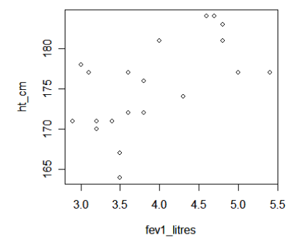
As an example of a study examining the association between two measurement variables, we will look at the association between forced expiratory volume (FEV1, a measure of lung function) and height (measured in centimeters) in a sample of 20 young adults. Data for the first 5 subjects:
|
ID |
sexM |
ht_cm |
fev1_litres |
|---|---|---|---|
|
1 |
1 |
174 |
4.3 |
|
2 |
1 |
181 |
4.8 |
|
3 |
0 |
184 |
4.7 |
|
4 |
1 |
177 |
5.4 |
|
5 |
1 |
177 |
3.1 |
The plot( ) function will graph a scatter plot. To plot FEV1 (the dependent or outcome variable) on the Y axis, and height (the independent or predictor variable) on the X axis:
> plot(ht_cm ~ fev1_litres)
The 'cor( )' function calculates correlation coefficients between the variables in a data set (vectors in a matrix object). For our height and lung function example, where 'fevheight' is the matrix object representing the data set:
> cor(fevheight)
ID sexM ht_cm fev1_litres
ID 1.00000000 0.02726935 -0.1624661 -0.4339991
sexM 0.02726935 1.00000000 0.1044337 -0.1196384
ht_cm -0.16246613 0.10443368 1.0000000 0.5973320
fev1_litres -0.43399905 -0.11963840 0.5973320 1.0000000
The 'cor.test( )' function gives more detail around the correlation coefficient between two measurement variables, testing the null hypothesis of zero correlation (no association) and giving a CI for the correlation coefficient. For our height and lung function example:
> cor.test(ht_cm,fev1_litres)
Pearson's product-moment correlation
data: ht_cm and fev1_litres
t = 3.16, df = 18, p-value = 0.005419
alternative hypothesis: true correlation is not equal to 0
95 percent confidence interval:
0.2104363 0.8224525
sample estimates:
cor
0.597332
Regression analysis is performed through the 'lm( )' function. LM stands for Linear Models, and this function can be used to perform simple regression, multiple regression, and Analysis of Variance.
For simple regression (with just one independent or predictor variable), predicting FEV1 from height:
> summary(lm(fev1_litres ~ ht_cm) )
Call:
lm(formula = fev1_litres ~ ht_cm)
Residuals:
Min 1Q Median 3Q Max
-1.12043 -0.36014 -0.02043 0.32223 1.35898
Coefficients:
Estimate Std. Error t value Pr(>|t|)
(Intercept) -10.01429 4.40863 -2.272 0.03562 *
ht_cm 0.07941 0.02513 3.160 0.00542 **
---
Signif. codes: 0 '***' 0.001 '**' 0.01 '*' 0.05 '.' 0.1 ' ' 1
Residual standard error: 0.6148 on 18 degrees of freedom
Multiple R-Squared: 0.3568, Adjusted R-squared: 0.3211
F-statistic: 9.985 on 1 and 18 DF, p-value: 0.005419
The syntax here is actually calling two functions, the lm( ) function performs the regression analysis, and the summary( ) function prints selected output from the regression. The 'Estimate' column in the output gives the intercept and slope for the regression:
fev1 = -10.014 + 0.079 (ht_cm).
The Pr(>|t|) column in the output gives the p-value for the slope. Here, the p-value for the slope for height is .00542.
The cor.test( ) function that calculates the usual Pearson's correlation will also calculate Spearman's nonparametric correlation coefficient (rho). With small samples and no ties, an exact p-value is calculated, otherwise a normal approximation is used to calculate the p-value. In this example, Lactate and Alanine are two variables measured on a sample of n=16 subjects.
> cor.test(Lactate,Alanine,method='spearman')
Spearman's rank correlation rho
data: Lactate and Alanine
S = 196, p-value = 0.002663
alternative hypothesis: true rho is not equal to 0
sample estimates:
rho
0.7117647
Multiple regression analysis is also performed through the 'lm( )' function. The syntax is the same as for simple regression except that more than one predictor variable is specified:
> summary(lm(fev1_litres ~ ht_cm + sexM))
Call:
lm(formula = fev1_litres ~ ht_cm + sexM)
Residuals:
Min 1Q Median 3Q Max
-1.02900 -0.33864 -0.08322 0.36404 1.45297
Coefficients:
Estimate Std. Error t value Pr(>|t|)
(Intercept) -10.27991 4.42528 -2.323 0.03284 *
ht_cm 0.08196 0.02531 3.238 0.00484 **
sexM -0.28059 0.29034 -0.966 0.34738
---
Signif. codes: 0 '***' 0.001 '**' 0.01 '*' 0.05 '.' 0.1 ' ' 1
Residual standard error: 0.6159 on 17 degrees of freedom
Multiple R-Squared: 0.3903, Adjusted R-squared: 0.3186
F-statistic: 5.441 on 2 and 17 DF, p-value: 0.01491
In regression analyses, categorical predictors are represented through a set of 0/1 indicator (or dummy) variables. The factor( ) command in R identifies categorical variables and creates dummy variables for a categorical variable. For example, the variable 'bmicat' is coded 1, 2, 3, 4 to indicate those who are underweight, normal weight, overweight, or obese. In creating dummy variables, the factor( ) command chooses the lowest coded category as the reference category, so here will choose 'underweight' as the reference group (see below to see how to change the reference category). The factor( ) command can be used inside the lm( ) command to indicate categorical predicators:
> summary(lm(sysbp ~ age + studygrp + factor(bmicat)))
Call:
lm(formula = sysbp ~ age + studygrp + factor(BMIcat))
Residuals:
Min 1Q Median 3Q Max
-38.276 -8.802 -1.720 6.922 56.383
Coefficients:
Estimate Std. Error t value Pr(>|t|)
(Intercept) 55.9938 12.6939 4.411 2.00e-05 ***
age 0.6676 0.1065 6.266 4.04e-09 ***
studygrp 4.4550 2.6644 1.672 0.096681 .
factor(BMIcat)2 30.3576 11.0720 2.742 0.006885 **
factor(BMIcat)3 32.4454 11.0745 2.930 0.003946 **
factor(BMIcat)4 45.8055 12.3038 3.723 0.000282 ***
---
Signif. codes: 0 '***' 0.001 '**' 0.01 '*' 0.05 '.' 0.1 ' ' 1
Residual standard error: 15.29 on 144 degrees of freedom
Multiple R-squared: 0.2884, Adjusted R-squared: 0.2637
F-statistic: 11.67 on 5 and 144 DF, p-value: 1.767e-09
Note that three dummy variable were included in the regression representing the four bmi categories.
In this example, it would be more natural to use 'normal weight', which is coded as BMIcat of 2, as the reference group. You can specify the reference group for a categorical variable with the 'relevel( )' command (for reference level, I think). Here, to specify '2' as the reference category, we would use relevel(factor(BMIcat,ref="2")) (getting a bit involved, using R functions within functions within functions):
> summary(lm(sysbp ~ age + studygrp + relevel(factor(BMIcat),ref="2")))
Call:
lm(formula = sysbp ~ age + studygrp + relevel(factor(BMIcat), ref = "2"))
Coefficients:
Estimate Std. Error t value Pr(>|t|)
(Intercept) 86.3514 6.1109 14.131 < 2e-16 ***
age 0.6676 0.1065 6.266 4.04e-09 ***
studygrp 4.4550 2.6644 1.672 0.09668 .
relevel(factor(BMIcat), ref = "2")1 -30.3576 11.0720 -2.742 0.00689 **
relevel(factor(BMIcat), ref = "2")3 2.0878 2.6448 0.789 0.43118
relevel(factor(BMIcat), ref = "2")4 15.4479 6.0609 2.549 0.01186 *
---
Signif. codes: 0 '***' 0.001 '**' 0.01 '*' 0.05 '.' 0.1 ' ' 1
Residual standard error: 15.29 on 144 degrees of freedom
Multiple R-squared: 0.2884, Adjusted R-squared: 0.2637
F-statistic: 11.67 on 5 and 144 DF, p-value: 1.767e-09
These results use normal weight as the reference category.
R gives (unstandardized) regression coefficients and the model R-square as part of the standard output from a regression analysis, but does not include the standardized regression coefficients as part of the standard output.
For example, the following regression model predicts systolic blood pressure from sex, age, BMI, and cholesterol levels:
> summary(lm(SYSBP ~ AGE + SEX + BMI + TOTCHOL))
Call:
lm(formula = SYSBP ~ AGE + SEX + BMI + TOTCHOL)
Coefficients:
Estimate Std. Error t value Pr(>|t|)
(Intercept) 40.98768 11.81398 3.469 0.000642 ***
AGE 0.89031 0.16052 5.546 9.41e-08 ***
SEX 5.49818 2.81491 1.953 0.052222 .
BMI 1.43825 0.29289 4.910 1.92e-06 ***
TOTCHOL 0.00636 0.03330 0.191 0.848733
---
Signif. codes: 0 '***' 0.001 '**' 0.01 '*' 0.05 '.' 0.1 ' ' 1
Residual standard error: 19.19 on 195 degrees of freedom
Multiple R-squared: 0.2879, Adjusted R-squared: 0.2733
F-statistic: 19.71 on 4 and 195 DF, p-value: 1.219e-13
One way to calculate standardized regression coefficients in R is to do it 'by hand'. The to find the standardized coefficients, we can first convert every variable in the analysis to a z-score, using the 'scale' function (I've named these new z-score variables with a '.z' as a reminder that these are z-scores, but this is not necessary, and it's not necessary):
> sysbp.z <- scale(SYSBP)
> age.z <- scale(AGE)
> sex.z <- scale(SEX)
> bmi.z <- scale(BMI)
> totchol.z <- scale(TOTCHOL)
Just to check, the mean for these z-score variables should be 0 and the standard deviation should be 1:
> mean(totchol.z)
[1] -2.196409e-16
> sd(totchol.z)
[1] 1
We can find the standardized coefficients by running the regression analysis on the z-score version of the variables:
> summary(lm(sysbp.z ~ age.z + sex.z + bmi.z + totchol.z))
Call:
lm(formula = sysbp.z ~ age.z + sex.z + bmi.z + totchol.z)
Residuals:
Min 1Q Median 3Q Max
-1.7566 -0.6151 -0.1565 0.5738 3.2835
Coefficients:
Estimate Std. Error t value Pr(>|t|)
(Intercept) 1.902e-16 6.028e-02 3.15e-15 1.0000
age.z 3.529e-01 6.363e-02 5.546 9.41e-08 ***
sex.z 1.200e-01 6.141e-02 1.953 0.0522 .
bmi.z 3.030e-01 6.170e-02 4.910 1.92e-06 ***
totchol.z 1.188e-02 6.223e-02 0.191 0.8487
---
Signif. codes: 0 '***' 0.001 '**' 0.01 '*' 0.05 '.' 0.1 ' ' 1
Residual standard error: 0.8525 on 195 degrees of freedom
Multiple R-squared: 0.2879, Adjusted R-squared: 0.2733
F-statistic: 19.71 on 4 and 195 DF, p-value: 1.219e-13
The 'slopes' from this analysis are the standardized slopes. Note that the p-values for the (now standardized) slopes match the p-values from the original version of the analysis, and that the model R-square is the same as in the original version of the analysis.\
In R, logistic regression is performed using the glm( ) function, for general linear model. This function can fit several regression models, and the syntax specifies the request for a logistic regression model.
As an example, we will look at factors associated with smoking among a sample of n=300 high school students from the Youth Risk Behavior Survey. The outcome variable is 'eversmokedaily1', coded as 1 for those who have smoked vs. 0 for those who have not. As a preliminary analysis, we calculate the proportion of respondents who have ever smoked daily:
> table(eversmokedaily1)
eversmokedaily1
0 1
229 69
> 69/(69+229)
[1] 0.2315436
In the following example, the glm( ) function performs the logistic regression, and the summary( ) function requests the default output summarizing the analysis. The 'family=binomial(link=logit)' syntax specifies a logistic regression model. As with the linear regression routine and the ANOVA routine in R, the 'factor( )' command can be used to declare a categorical predictor (with more than two categories) in a logistic regression; R will create dummy variables to represent the categorical predictor using the lowest coded category as the reference group.
In entering this command, I hit the 'return' to type things in over 2 lines; R will allow you to continue a command onto a second or third line.
In this example, 'bmi_cat' is a categorical variable coded 1,2,3 or 4 for those in BMI categories of underweight, normal weight, overweight, or obese. By default, R creates 3 dummy variables to represent BMI category, using the lowest coded group (here 'underweight') as the reference. You can change the reference category by using the 'relevel( )' command (see dummy variables in multiple linear regression, above). The format of the relevel( ) command is:
relevel(factor(bmi_cat,ref="2")
This command would treat bmi_cat as a categorical predictor, and use category '2' (normal weight) as the reference category when creating dummy variables:
> summary(glm(eversmokedaily1 ~ age + sex1F2M +
relevel(factor(bmi_cat),ref='2') + alc_30days,
family=binomial(link=logit)))
Call:
glm(formula = eversmokedaily1 ~ age + sex1F2M + relevel(factor(bmi_cat),
ref = "2") + alc_30days, family = binomial(link = logit))
Deviance Residuals:
Min 1Q Median 3Q Max
-1.2067 -0.8476 -0.3406 -0.1983 2.5519
Coefficients:
Estimate Std. Error z value Pr(>|z|)
(Intercept) -2.46565 1.98469 -1.242 0.2141
age -0.07688 0.12163 -0.632 0.5273
sex1F2M 0.55572 0.32236 1.724 0.0847 .
relevel(factor(bmi_cat), ref = "2")1 0.24505 0.55573 0.441 0.6593
relevel(factor(bmi_cat), ref = "2")3 0.19814 0.40889 0.485 0.6280
relevel(factor(bmi_cat), ref = "2")4 -0.70254 0.60298 -1.165 0.2440
alc_30days 2.30101 0.45628 5.043 4.58e-07 ***
---
Signif. codes: 0 '***' 0.001 '**' 0.01 '*' 0.05 '.' 0.1 ' ' 1
(Dispersion parameter for binomial family taken to be 1)
Null deviance: 292.83 on 268 degrees of freedom
Residual deviance: 247.20 on 262 degrees of freedom
(31 observations deleted due to missingness)
AIC: 261.20
Number of Fisher Scoring iterations: 5
In logistic regression, slopes can be converted to odds ratios for interpretation. Below we calculate the odds ratio for those in the BMI overweight category, and we calculate the OR and the 95% CI for the OR for those having had a drink in the past month vs. those not having had a drink in the past month (the # indicates a comment that is ignored by R):
> exp(0.55572) #OR for males compared to females
[1] 1.743196
> exp(0.55572 - 1.96*0.32236) # lower limit of 95% CI for OR
[1] 0.9267183
> exp(0.55572 + 1.96*0.32236) # upper limit of 95% CI for OR
[1] 3.279023
The C-statistic (also called the AUC statistic) for the logistic regression can be obtained from the lroc( ) command, which is in the 'epicalc' add-on package. To find the C-statistic, you must first install and then load the epicalc package. Once the package is loaded, you can find the C-statistic by first saving the results of the logistic regression, and then using the lroc( ) command:
> logisticresults <- glm(eversmokedaily1 ~ age + sex1F2M, family=binomial(link=logit)))
> lroc(logisticresults)
$model.description
[1] "eversmokedaily1 ~ age + sex1F2M"
$auc
[1] 0.5787582
The lroc( ) command gives a lot of additional output (more detail than we generally need) and a graph of the ROC curve; the C-statistic is given at the top of the output, labeled 'auc'.
Survival analyses can be performed using the 'survival' add-on package in R (see Section 16d to download the package into R). First, load 'survival' into the R session by clicking on the Packages menu, then Load Packages and selecting survival.
The 'survfit' function from the 'survival' add-on package calculates and plots the Kaplan-Meier survival curve, and also calculates median survival from the Kaplan-Meier curve. The following example analyzes survival for 13 people who were exposed to large doses of radiation during the Chernobyl nuclear accident and received bone marrow transplants (Baranov et.al., NEJM, 1989). The input for the 'survfit( )' function include a variable containing survival/censoring time (days.surv in this example) and an indicator variable for event (coded 1) or censored (coded 0) (death in this example). The 'summary( )' function with survfit gives a listing of the survival function, the 'print( )' function with survfit gives the median survival with a 95% CI, and the 'plot( )' function with survfit gives a plot of the K-M curve with a 95% confidence band (while all 3 functions are illustrated below, it is not necessary to run all three – the K-M plot could be requested directly without printing out the survival proportions).
> summary(survfit(Surv(days.surv,death)))
Call: survfit(formula = Surv(days.surv, death))
time n.risk n.event survival std.err lower 95% CI upper 95% CI
15 13 1 0.923 0.0739 0.7890 1.000
17 12 1 0.846 0.1001 0.6711 1.000
18 11 2 0.692 0.1280 0.4819 0.995
23 9 1 0.615 0.1349 0.4004 0.946
24 8 1 0.538 0.1383 0.3255 0.891
25 7 1 0.462 0.1383 0.2566 0.830
34 6 1 0.385 0.1349 0.1934 0.765
48 5 1 0.308 0.1280 0.1361 0.695
86 4 1 0.231 0.1169 0.0855 0.623
91 3 1 0.154 0.1001 0.0430 0.550
> print(survfit(Surv(days.surv,death)))
Call: survfit(formula = Surv(days.surv, death))
n events median 0.95LCL 0.95UCL
13 11 25 18 Inf
> plot(survfit(Surv(days.surv,death)))
The 'print( )', 'plot( )', and 'survdiff( )' functions in the 'survival' add-ono package can be used to compare median survival times, plot K-M survival curves by group, and perform the log-rank test to compare two groups on survival. In the following example, 'survmonths' is survival time in months, 'event' is an indicator variable coded 1 for those who have had the outcome event and 0 for those who are censored, and 'group' is an indicator variable coded 1 for the experimental and 0 for the control group.
> print(survfit(Surv(survmonths,event) ~ group))
Call: survfit(formula = Surv(survmonths, event) ~ group)
n events median 0.95LCL 0.95UCL
group=0 28 22 4 3 5
group=1 22 12 14 6 Inf
> plot(survfit(Surv(survmonths,event) ~ group))
> survdiff(Surv(survmonths,event) ~ group)
Call:
survdiff(formula = Surv(survmonths, event) ~ group)
N Observed Expected (O-E)^2/E (O-E)^2/V
group=0 28 22 11.3 10.05 20.7
group=1 22 12 22.7 5.02 20.7
Chisq= 20.7 on 1 degrees of freedom, p= 5.33e-06
The chi-square statistic and p-value given above are for the log rank test of the null hypothesis of no difference between the two survival curves.
Cox's proportional hazards regression can be performed using the 'coxph( )' and 'Surv( )' functions of the 'survival' add –on package. R gives the parameter estimates for the Cox model, which can be exponentiated to give estimated hazard ratios (HRs), and confidence intervals for the parameter estimates can be used to get confidence intervals for the hazards ratios. The following performs a proportional hazards regression predicting survival from treatment group (coded 0,1) and age in years, and then finds the HR and 95% CI for the HR comparing groups.
The 'factor( )' function can be used to declare multi-category categorical predictors in a Cox model (to be represented by dummy variables in the model), and the 'relevel(factor( ), ref='') command can be used to specify the reference category in creating dummy variables (see the examples under multiple linear regression and multiple logistic regression above).
> coxph(Surv(survmonths,event) ~ group+age)
Call:
coxph(formula = Surv(survmonths, event) ~ group + age)
coef exp(coef) se(coef) z p
group -1.94034 0.144 0.4872 -3.982 6.8e-05
age 0.00963 1.010 0.0321 0.300 7.6e-01
Likelihood ratio test=20.5 on 2 df, p=3.61e-05 n= 50
> exp(-1.94034)
[1] 0.1436551
> exp(-1.94034-1.93*0.144)
[1] 0.1087983
> exp(-1.94034+1.93*0.144)
[1] 0.1896794
Here, group is significantly related to survival (p<.001), with better survival in the treatment group (group=1) than control group (group=0), with HR=0.143, 95% CI (0.019 , 0.190). Age does not significantly relate to survival (p=0.76).
For studies with multiple outcomes, p-values can be adjusted to account for the multiple comparisons issue. The 'p.adjust( )' command in R calculates adjusted p-values from a set of un-adjusted p-values, using a number of adjustment procedures.
Adjustment procedures that give strong control of the family-wise error rate are the Bonferroni, Holm, Hochberg, and Hommel procedures.
Adjustments that control for the false discovery rate, which is the expected proportion of false discoveries among the rejected hypotheses, are the Benjamini and Hochberg, and Benjamini, Hochberg, and Yekutieli procedures.
To calculate adjusted p-values, first save a vector of un-adjusted p-values. The following example is from a study comparing two groups on 10 outcomes through t-tests and chi-square tests, where 3 of the outcomes gave un-adjusted p-values below the conventional 0.05 level. The following calculates adjusted p-values using the Bonferroni, Hochberg, and Benjamini and Hochberg (BH) methods:
> pvalues <- c(.002, .005, .015, .113, .222, .227, .454, .552, .663, .751)
> p.adjust(pvalues,method="bonferroni")
[1] 0.02 0.05 0.15 1.00 1.00 1.00 1.00 1.00 1.00 1.00
> p.adjust(pvalues,method="hochberg")
[1] 0.020 0.045 0.120 0.751 0.751 0.751 0.751 0.751 0.751 0.751
> p.adjust(pvalues,method="BH")
[1] 0.0200000 0.0250000 0.0500000 0.2825000 0.3783333 0.3783333 0.6485714
[8] 0.6900000 0.7366667 0.7510000
Other adjustments can be requested using "holm", "hommel", and "BY" (for the Benjamini, Hochber, and Yekutieli procedure).
User-defined functions can also be created and saved in R. As a simple example, the following code creates a user-defined function to calculate a 95% confidence interval for a proportion. The function name is 'CIp', and the input for the function is p (the sample proportion) and n (the sample size). The '+'s at the beginning of lines were typed by R and indicate a continuation of the previous line/calculation. The '{ }'s in the function specification indicate individual calculations or function calls within the function. 'cresult' is a column vector containing lower (p.lower) and upper (p.upper) confidence limits, and the 'return( )' function indicates which of the objects created in the function are to be printed when the function is called.
> CIp <- function(p,n) {
+ {p.lower <- p-1.96*sqrt(p*(1-p)/n)}
+ {p.upper <- p+1.96*sqrt(p*(1-p)/n)}
+ {cresult <- c(p.lower,p.upper)}
+ return(cresult)
+ }
> CIp(.30,100)
[1] 0.2101815 0.3898185
> CIp(.3,1000)
[1] 0.2715969 0.3284031
The following creates a function to calculate two-tailed p-values from a t-statistic. The cat( ) function specifies the print out. Unlike the return( ) function (I think), cat( ) allows text labels to be included in quotes and more than one object to be printed on a line. The '\n' in the cat( ) function inserts a line return after printing the label and p-value, and multiple line returns could be specified in a cat( ) statement.
> pvalue.t <- function(t,df) {
+ pval <- 2*(1-pt(abs(t),df))
+ cat('Two-tailed p-value',pval,'\n')
+ }
> pvalue.t(2.33,200)
Two-tailed p-value 0.02080349
> pvalue.t(-1.55,45)
Two-tailed p-value 0.1281466