


Section 4: Association between variables and multivariable methods to control for confounding
4.1 Simple correlation and regression
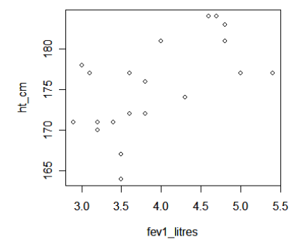
As an example of a study examining the association between two measurement variables, we will look at the association between forced expiratory volume (FEV1, a measure of lung function) and height (measured in centimeters) in a sample of 20 young adults. Data for the first 5 subjects:
|
ID |
sexM |
ht_cm |
fev1_litres |
|---|---|---|---|
|
1 |
1 |
174 |
4.3 |
|
2 |
1 |
181 |
4.8 |
|
3 |
0 |
184 |
4.7 |
|
4 |
1 |
177 |
5.4 |
|
5 |
1 |
177 |
3.1 |
4.1.1 Scatterplots
The plot( ) function will graph a scatter plot. To plot FEV1 (the dependent or outcome variable) on the Y axis, and height (the independent or predictor variable) on the X axis:
> plot(ht_cm ~ fev1_litres)
4.1.2 Correlation
The 'cor( )' function calculates correlation coefficients between the variables in a data set (vectors in a matrix object). For our height and lung function example, where 'fevheight' is the matrix object representing the data set:
> cor(fevheight)
ID sexM ht_cm fev1_litres
ID 1.00000000 0.02726935 -0.1624661 -0.4339991
sexM 0.02726935 1.00000000 0.1044337 -0.1196384
ht_cm -0.16246613 0.10443368 1.0000000 0.5973320
fev1_litres -0.43399905 -0.11963840 0.5973320 1.0000000
The 'cor.test( )' function gives more detail around the correlation coefficient between two measurement variables, testing the null hypothesis of zero correlation (no association) and giving a CI for the correlation coefficient. For our height and lung function example:
> cor.test(ht_cm,fev1_litres)
Pearson's product-moment correlation
data: ht_cm and fev1_litres
t = 3.16, df = 18, p-value = 0.005419
alternative hypothesis: true correlation is not equal to 0
95 percent confidence interval:
0.2104363 0.8224525
sample estimates:
cor
0.597332
4.1.3 Simple regression analysis
Regression analysis is performed through the 'lm( )' function. LM stands for Linear Models, and this function can be used to perform simple regression, multiple regression, and Analysis of Variance.
For simple regression (with just one independent or predictor variable), predicting FEV1 from height:
> summary(lm(fev1_litres ~ ht_cm) )
Call:
lm(formula = fev1_litres ~ ht_cm)
Residuals:
Min 1Q Median 3Q Max
-1.12043 -0.36014 -0.02043 0.32223 1.35898
Coefficients:
Estimate Std. Error t value Pr(>|t|)
(Intercept) -10.01429 4.40863 -2.272 0.03562 *
ht_cm 0.07941 0.02513 3.160 0.00542 **
---
Signif. codes: 0 '***' 0.001 '**' 0.01 '*' 0.05 '.' 0.1 ' ' 1
Residual standard error: 0.6148 on 18 degrees of freedom
Multiple R-Squared: 0.3568, Adjusted R-squared: 0.3211
F-statistic: 9.985 on 1 and 18 DF, p-value: 0.005419
The syntax here is actually calling two functions, the lm( ) function performs the regression analysis, and the summary( ) function prints selected output from the regression. The 'Estimate' column in the output gives the intercept and slope for the regression:
fev1 = -10.014 + 0.079 (ht_cm).
The Pr(>|t|) column in the output gives the p-value for the slope. Here, the p-value for the slope for height is .00542.
4.1.4 Spearman's nonparametric correlation coefficient
The cor.test( ) function that calculates the usual Pearson's correlation will also calculate Spearman's nonparametric correlation coefficient (rho). With small samples and no ties, an exact p-value is calculated, otherwise a normal approximation is used to calculate the p-value. In this example, Lactate and Alanine are two variables measured on a sample of n=16 subjects.
> cor.test(Lactate,Alanine,method='spearman')
Spearman's rank correlation rho
data: Lactate and Alanine
S = 196, p-value = 0.002663
alternative hypothesis: true rho is not equal to 0
sample estimates:
rho
0.7117647