


The ANOVA Approach
Consider an example with four independent groups and a continuous outcome measure. The independent groups might be defined by a particular characteristic of the participants such as BMI (e.g., underweight, normal weight, overweight, obese) or by the investigator (e.g., randomizing participants to one of four competing treatments, call them A, B, C and D). Suppose that the outcome is systolic blood pressure, and we wish to test whether there is a statistically significant difference in mean systolic blood pressures among the four groups. The sample data are organized as follows:
|
|
Group 1 |
Group 2 |
Group 3 |
Group 4 |
|---|---|---|---|---|
|
Sample Size |
n1 |
n2 |
n3 |
n4 |
|
Sample Mean |
|
|
|
|
|
Sample Standard Deviation |
s1 |
s2 |
s3 |
s4 |


The hypotheses of interest in an ANOVA are as follows:
- H0: μ1 = μ2 = μ3 ... = μk
- H1: Means are not all equal.
where k = the number of independent comparison groups.
In this example, the hypotheses are:
- H0: μ1 = μ2 = μ3 = μ4
- H1: The means are not all equal.
The null hypothesis in ANOVA is always that there is no difference in means. The research or alternative hypothesis is always that the means are not all equal and is usually written in words rather than in mathematical symbols. The research hypothesis captures any difference in means and includes, for example, the situation where all four means are unequal, where one is different from the other three, where two are different, and so on. The alternative hypothesis, as shown above, capture all possible situations other than equality of all means specified in the null hypothesis.
Test Statistic for ANOVA
The test statistic for testing H0: μ1 = μ2 = ... = μk is:

and the critical value is found in a table of probability values for the F distribution with (degrees of freedom) df1 = k-1, df2=N-k. The table can be found in "Other Resources" on the left side of the pages.
In the test statistic, nj = the sample size in the jth group (e.g., j =1, 2, 3, and 4 when there are 4 comparison groups),  is the sample mean in the jth group, and
  is the overall mean. k represents the number of independent groups (in this example, k=4), and N represents the total number of observations in the analysis. Note that N does not refer to a population size, but instead to the total sample size in the analysis (the sum of the sample sizes in the comparison groups, e.g., N=n1+n2+n3+n4). The test statistic is complicated because it incorporates all of the sample data. While it is not easy to see the extension, the F statistic shown above is a generalization of the test statistic used for testing the equality of exactly two means.
NOTE: The test statistic F assumes equal variability in the k populations (i.e., the population variances are equal, or s12 = s22 = ... = sk2 ). This means that the outcome is equally variable in each of the comparison populations. This assumption is the same as that assumed for appropriate use of the test statistic to test equality of two independent means. It is possible to assess the likelihood that the assumption of equal variances is true and the test can be conducted in most statistical computing packages. If the variability in the k comparison groups is not similar, then alternative techniques must be used.
The F statistic is computed by taking the ratio of what is called the "between treatment" variability to the "residual or error" variability. This is where the name of the procedure originates. In analysis of variance we are testing for a difference in means (H0: means are all equal versus H1: means are not all equal) by evaluating variability in the data. The numerator captures between treatment variability (i.e., differences among the sample means) and the denominator contains an estimate of the variability in the outcome. The test statistic is a measure that allows us to assess whether the differences among the sample means (numerator) are more than would be expected by chance if the null hypothesis is true. Recall in the two independent sample test, the test statistic was computed by taking the ratio of the difference in sample means (numerator) to the variability in the outcome (estimated by Sp).
The decision rule for the F test in ANOVA is set up in a similar way to decision rules we established for t tests. The decision rule again depends on the level of significance and the degrees of freedom. The F statistic has two degrees of freedom. These are denoted df1 and df2, and called the numerator and denominator degrees of freedom, respectively. The degrees of freedom are defined as follows:
df1 = k-1 and df2=N-k,
where k is the number of comparison groups and N is the total number of observations in the analysis. If the null hypothesis is true, the between treatment variation (numerator) will not exceed the residual or error variation (denominator) and the F statistic will small. If the null hypothesis is false, then the F statistic will be large. The rejection region for the F test is always in the upper (right-hand) tail of the distribution as shown below.
Rejection Region for F Test with a =0.05, df1=3 and df2=36 (k=4, N=40)
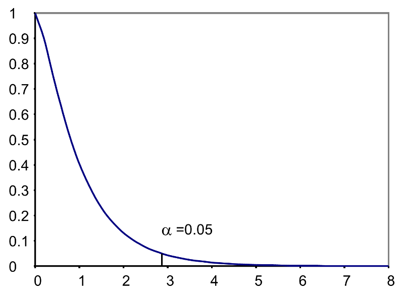
For the scenario depicted here, the decision rule is: Reject H0 if F > 2.87.