


Summary
Here we presented hypothesis testing techniques for means and proportions in one and two sample situations. Tests of hypothesis involve several steps, including specifying the null and alternative or research hypothesis, selecting and computing an appropriate test statistic, setting up a decision rule and drawing a conclusion. There are many details to consider in hypothesis testing. The first is to determine the appropriate test. We discussed Z and t tests here for different applications. The appropriate test depends on the distribution of the outcome variable (continuous or dichotomous), the number of comparison groups (one, two) and whether the comparison groups are independent or dependent. The following table summarizes the different tests of hypothesis discussed here.
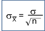
- Continuous Outcome, One Sample: H0: μ = μ0


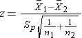
- Continuous Outcome, Two Independent Samples: H0: μ1 = μ2
and 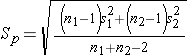
- Continuous Outcome, Two Matched Samples: H0: μd = 0

and

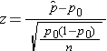
- Dichotomous Outcome, One Sample: H0: p = p 0
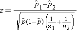
- Dichotomous Outcome, Two Independent Samples: H0: p1 = p2, RD=0, RR=1, OR=1
Once the type of test is determined, the details of the test must be specified. Specifically, the null and alternative hypotheses must be clearly stated. The null hypothesis always reflects the "no change" or "no difference" situation. The alternative or research hypothesis reflects the investigator's belief. The investigator might hypothesize that a parameter (e.g., a mean, proportion, difference in means or proportions) will increase, will decrease or will be different under specific conditions (sometimes the conditions are different experimental conditions and other times the conditions are simply different groups of participants). Once the hypotheses are specified, data are collected and summarized. The appropriate test is then conducted according to the five step approach. If the test leads to rejection of the null hypothesis, an approximate p-value is computed to summarize the significance of the findings. When tests of hypothesis are conducted using statistical computing packages, exact p-values are computed. Because the statistical tables in this textbook are limited, we can only approximate p-values. If the test fails to reject the null hypothesis, then a weaker concluding statement is made for the following reason.
In hypothesis testing, there are two types of errors that can be committed. A Type I error occurs when a test incorrectly rejects the null hypothesis. This is referred to as a false positive result, and the probability that this occurs is equal to the level of significance, α. The investigator chooses the level of significance in Step 1, and purposely chooses a small value such as α=0.05 to control the probability of committing a Type I error. A Type II error occurs when a test fails to reject the null hypothesis when in fact it is false. The probability that this occurs is equal to β. Unfortunately, the investigator cannot specify β at the outset because it depends on several factors including the sample size (smaller samples have higher b), the level of significance (β decreases as a increases), and the difference in the parameter under the null and alternative hypothesis.
We noted in several examples in this chapter, the relationship between confidence intervals and tests of hypothesis. The approaches are different, yet related. It is possible to draw a conclusion about statistical significance by examining a confidence interval. For example, if a 95% confidence interval does not contain the null value (e.g., zero when analyzing a mean difference or risk difference, one when analyzing relative risks or odds ratios), then one can conclude that a two-sided test of hypothesis would reject the null at α=0.05. It is important to note that the correspondence between a confidence interval and test of hypothesis relates to a two-sided test and that the confidence level corresponds to a specific level of significance (e.g., 95% to α=0.05, 90% to α=0.10 and so on). The exact significance of the test, the p-value, can only be determined using the hypothesis testing approach and the p-value provides an assessment of the strength of the evidence and not an estimate of the effect.