


Introduction to Hypothesis Testing
Techniques for Hypothesis Testing
The techniques for hypothesis testing depend on
- the type of outcome variable being analyzed (continuous, dichotomous, discrete)
- the number of comparison groups in the investigation
- whether the comparison groups are independent (i.e., physically separate such as men versus women) or dependent (i.e., matched or paired such as pre- and post-assessments on the same participants).
In estimation we focused explicitly on techniques for one and two samples and discussed estimation for a specific parameter (e.g., the mean or proportion of a population), for differences (e.g., difference in means, the risk difference) and ratios (e.g., the relative risk and odds ratio). Here we will focus on procedures for one and two samples when the outcome is either continuous (and we focus on means) or dichotomous (and we focus on proportions).
General Approach: A Simple Example
The Centers for Disease Control (CDC) reported on trends in weight, height and body mass index from the 1960's through 2002.1 The general trend was that Americans were much heavier and slightly taller in 2002 as compared to 1960; both men and women gained approximately 24 pounds, on average, between 1960 and 2002. In 2002, the mean weight for men was reported at 191 pounds. Suppose that an investigator hypothesizes that weights are even higher in 2006 (i.e., that the trend continued over the subsequent 4 years). The research hypothesis is that the mean weight in men in 2006 is more than 191 pounds. The null hypothesis is that there is no change in weight, and therefore the mean weight is still 191 pounds in 2006.
|
Null Hypothesis |
H0: μ= 191 (no change) |
|
Research Hypothesis |
H1: μ> 191 (investigator's belief) |
In order to test the hypotheses, we select a random sample of American males in 2006 and measure their weights. Suppose we have resources available to recruit n=100 men into our sample. We weigh each participant and compute summary statistics on the sample data. Suppose in the sample we determine the following:
- n=100


- s=25.6
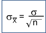
Do the sample data support the null or research hypothesis? The sample mean of 197.1 is numerically higher than 191. However, is this difference more than would be expected by chance? In hypothesis testing, we assume that the null hypothesis holds until proven otherwise. We therefore need to determine the likelihood of observing a sample mean of 197.1 or higher when the true population mean is 191 (i.e., if the null hypothesis is true or under the null hypothesis). We can compute this probability using the Central Limit Theorem. Specifically,

(Notice that we use the sample standard deviation in computing the Z score. This is generally an appropriate substitution as long as the sample size is large, n > 30. Thus, there is less than a 1% probability of observing a sample mean as large as 197.1 when the true population mean is 191. Do you think that the null hypothesis is likely true? Based on how unlikely it is to observe a sample mean of 197.1 under the null hypothesis (i.e., <1% probability), we might infer, from our data, that the null hypothesis is probably not true.
Suppose that the sample data had turned out differently. Suppose that we instead observed the following in 2006:
- n=100

- s=25.6
How likely it is to observe a sample mean of 192.1 or higher when the true population mean is 191 (i.e., if the null hypothesis is true)? We can again compute this probability using the Central Limit Theorem. Specifically,

There is a 33.4% probability of observing a sample mean as large as 192.1 when the true population mean is 191. Do you think that the null hypothesis is likely true?
Neither of the sample means that we obtained allows us to know with certainty whether the null hypothesis is true or not. However, our computations suggest that, if the null hypothesis were true, the probability of observing a sample mean >197.1 is less than 1%. In contrast, if the null hypothesis were true, the probability of observing a sample mean >192.1 is about 33%. We can't know whether the null hypothesis is true, but the sample that provided a mean value of 197.1 provides much stronger evidence in favor of rejecting the null hypothesis, than the sample that provided a mean value of 192.1. Note that this does not mean that a sample mean of 192.1 indicates that the null hypothesis is true; it just doesn't provide compelling evidence to reject it.
In essence, hypothesis testing is a procedure to compute a probability that reflects the strength of the evidence (based on a given sample) for rejecting the null hypothesis. In hypothesis testing, we determine a threshold or cut-off point (called the critical value) to decide when to believe the null hypothesis and when to believe the research hypothesis. It is important to note that it is possible to observe any sample mean when the true population mean is true (in this example equal to 191), but some sample means are very unlikely. Based on the two samples above it would seem reasonable to believe the research hypothesis when x̄ = 197.1, but to believe the null hypothesis when x̄ =192.1. What we need is a threshold value such that if x̄ is above that threshold then we believe that H1 is true and if x̄ is below that threshold then we believe that H0 is true. The difficulty in determining a threshold for x̄ is that it depends on the scale of measurement. In this example, the threshold, sometimes called the critical value, might be 195 (i.e., if the sample mean is 195 or more then we believe that H1 is true and if the sample mean is less than 195 then we believe that H0 is true). Suppose we are interested in assessing an increase in blood pressure over time, the critical value will be different because blood pressures are measured in millimeters of mercury (mmHg) as opposed to in pounds. In the following we will explain how the critical value is determined and how we handle the issue of scale.
First, to address the issue of scale in determining the critical value, we convert our sample data (in particular the sample mean) into a Z score. We know from the module on probability that the center of the Z distribution is zero and extreme values are those that exceed 2 or fall below -2. Z scores above 2 and below -2 represent approximately 5% of all Z values. If the observed sample mean is close to the mean specified in H0 (here m =191), then Z will be close to zero. If the observed sample mean is much larger than the mean specified in H0, then Z will be large.
In hypothesis testing, we select a critical value from the Z distribution. This is done by first determining what is called the level of significance, denoted α ("alpha"). What we are doing here is drawing a line at extreme values. The level of significance is the probability that we reject the null hypothesis (in favor of the alternative) when it is actually true and is also called the Type I error rate.
α = Level of significance = P(Type I error) = P(Reject H0 | H0 is true).
Because α is a probability, it ranges between 0 and 1. The most commonly used value in the medical literature for α is 0.05, or 5%. Thus, if an investigator selects α=0.05, then they are allowing a 5% probability of incorrectly rejecting the null hypothesis in favor of the alternative when the null is in fact true. Depending on the circumstances, one might choose to use a level of significance of 1% or 10%. For example, if an investigator wanted to reject the null only if there were even stronger evidence than that ensured with α=0.05, they could choose a =0.01as their level of significance. The typical values for α are 0.01, 0.05 and 0.10, with α=0.05 the most commonly used value.
Suppose in our weight study we select α=0.05. We need to determine the value of Z that holds 5% of the values above it (see below).
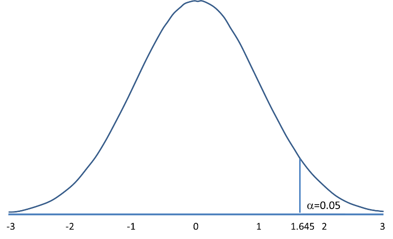
The critical value of Z for α =0.05 is Z = 1.645 (i.e., 5% of the distribution is above Z=1.645). With this value we can set up what is called our decision rule for the test. The rule is to reject H0 if the Z score is 1.645 or more.
With the first sample we have
Because 2.38 > 1.645, we reject the null hypothesis. (The same conclusion can be drawn by comparing the 0.0087 probability of observing a sample mean as extreme as 197.1 to the level of significance of 0.05. If the observed probability is smaller than the level of significance we reject H0). Because the Z score exceeds the critical value, we conclude that the mean weight for men in 2006 is more than 191 pounds, the value reported in 2002. If we observed the second sample (i.e., sample mean =192.1), we would not be able to reject the null hypothesis because the Z score is 0.43 which is not in the rejection region (i.e., the region in the tail end of the curve above 1.645). With the second sample we do not have sufficient evidence (because we set our level of significance at 5%) to conclude that weights have increased. Again, the same conclusion can be reached by comparing probabilities. The probability of observing a sample mean as extreme as 192.1 is 33.4% which is not below our 5% level of significance.