


Hypothesis Testing: Upper-, Lower, and Two Tailed Tests
The procedure for hypothesis testing is based on the ideas described above. Specifically, we set up competing hypotheses, select a random sample from the population of interest and compute summary statistics. We then determine whether the sample data supports the null or alternative hypotheses. The procedure can be broken down into the following five steps.
- Step 1. Set up hypotheses and select the level of significance α.
H0: Null hypothesis (no change, no difference);
H1: Research hypothesis (investigator's belief); α =0.05
|
Upper-tailed, Lower-tailed, Two-tailed Tests The research or alternative hypothesis can take one of three forms. An investigator might believe that the parameter has increased, decreased or changed. For example, an investigator might hypothesize:
The exact form of the research hypothesis depends on the investigator's belief about the parameter of interest and whether it has possibly increased, decreased or is different from the null value. The research hypothesis is set up by the investigator before any data are collected.
|
- Step 2. Select the appropriate test statistic.
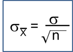
The test statistic is a single number that summarizes the sample information. An example of a test statistic is the Z statistic computed as follows:


When the sample size is small, we will use t statistics (just as we did when constructing confidence intervals for small samples). As we present each scenario, alternative test statistics are provided along with conditions for their appropriate use.
- Step 3. Set up decision rule.
The decision rule is a statement that tells under what circumstances to reject the null hypothesis. The decision rule is based on specific values of the test statistic (e.g., reject H0 if Z > 1.645). The decision rule for a specific test depends on 3 factors: the research or alternative hypothesis, the test statistic and the level of significance. Each is discussed below.
- The decision rule depends on whether an upper-tailed, lower-tailed, or two-tailed test is proposed. In an upper-tailed test the decision rule has investigators reject H0 if the test statistic is larger than the critical value. In a lower-tailed test the decision rule has investigators reject H0 if the test statistic is smaller than the critical value. In a two-tailed test the decision rule has investigators reject H0 if the test statistic is extreme, either larger than an upper critical value or smaller than a lower critical value.
- The exact form of the test statistic is also important in determining the decision rule. If the test statistic follows the standard normal distribution (Z), then the decision rule will be based on the standard normal distribution. If the test statistic follows the t distribution, then the decision rule will be based on the t distribution. The appropriate critical value will be selected from the t distribution again depending on the specific alternative hypothesis and the level of significance.
- The third factor is the level of significance. The level of significance which is selected in Step 1 (e.g., α =0.05) dictates the critical value. For example, in an upper tailed Z test, if α =0.05 then the critical value is Z=1.645.
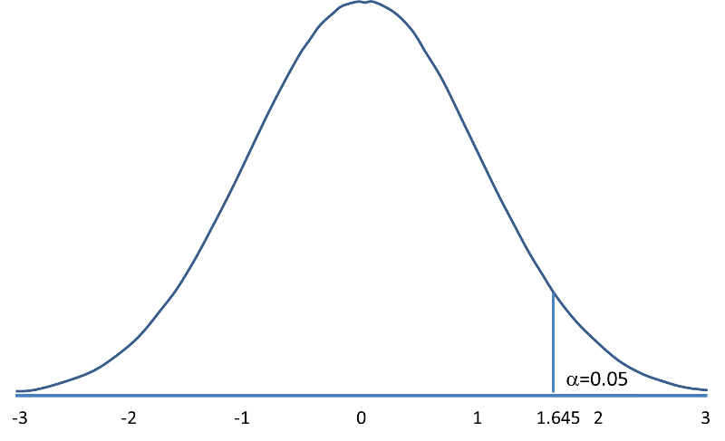
The following figures illustrate the rejection regions defined by the decision rule for upper-, lower- and two-tailed Z tests with α=0.05. Notice that the rejection regions are in the upper, lower and both tails of the curves, respectively. The decision rules are written below each figure.
|
Rejection Region for Upper-Tailed Z Test (H1: μ > μ0 ) with α=0.05 The decision rule is: Reject H0 if Z > 1.645. |
|
||||||||||||||||||
|
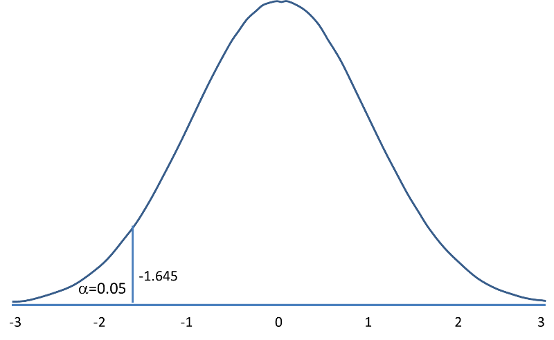
Rejection Region for Lower-Tailed Z Test (H1: μ < μ0 ) with α =0.05 The decision rule is: Reject H0 if Z < 1.645. |
|
||||||||||||||||||
|
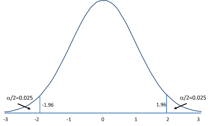
Rejection Region for Two-Tailed Z Test (H1: μ ≠ μ 0 ) with α =0.05 The decision rule is: Reject H0 if Z < -1.960 or if Z > 1.960. |
|
||||||||||||||||||
The complete table of critical values of Z for upper, lower and two-tailed tests can be found in the table of Z values to the right in "Other Resources."
Critical values of t for upper, lower and two-tailed tests can be found in the table of t values in "Other Resources."
- Step 4. Compute the test statistic.
Here we compute the test statistic by substituting the observed sample data into the test statistic identified in Step 2.
- Step 5. Conclusion.
The final conclusion is made by comparing the test statistic (which is a summary of the information observed in the sample) to the decision rule. The final conclusion will be either to reject the null hypothesis (because the sample data are very unlikely if the null hypothesis is true) or not to reject the null hypothesis (because the sample data are not very unlikely).
If the null hypothesis is rejected, then an exact significance level is computed to describe the likelihood of observing the sample data assuming that the null hypothesis is true. The exact level of significance is called the p-value and it will be less than the chosen level of significance if we reject H0.
Statistical computing packages provide exact p-values as part of their standard output for hypothesis tests. In fact, when using a statistical computing package, the steps outlined about can be abbreviated. The hypotheses (step 1) should always be set up in advance of any analysis and the significance criterion should also be determined (e.g., α =0.05). Statistical computing packages will produce the test statistic (usually reporting the test statistic as t) and a p-value. The investigator can then determine statistical significance using the following: If p < α then reject H0.
|
Things to Remember When Interpreting P Values
|
We now use the five-step procedure to test the research hypothesis that the mean weight in men in 2006 is more than 191 pounds. We will assume the sample data are as follows: n=100,  =197.1 and s=25.6.
- Step 1. Set up hypotheses and determine level of significance
H0: μ = 191 H1: μ > 191 α =0.05
The research hypothesis is that weights have increased, and therefore an upper tailed test is used.
- Step 2. Select the appropriate test statistic.
Because the sample size is large (n>30) the appropriate test statistic is
- Step 3. Set up decision rule.
In this example, we are performing an upper tailed test (H1: μ> 191), with a Z test statistic and selected α =0.05. Reject H0 if Z > 1.645.
- Step 4. Compute the test statistic.
We now substitute the sample data into the formula for the test statistic identified in Step 2.
- Step 5. Conclusion.
We reject H0 because 2.38 > 1.645. We have statistically significant evidence at a =0.05, to show that the mean weight in men in 2006 is more than 191 pounds. Because we rejected the null hypothesis, we now approximate the p-value which is the likelihood of observing the sample data if the null hypothesis is true. An alternative definition of the p-value is the smallest level of significance where we can still reject H0. In this example, we observed Z=2.38 and for α=0.05, the critical value was 1.645. Because 2.38 exceeded 1.645 we rejected H0. In our conclusion we reported a statistically significant increase in mean weight at a 5% level of significance. Using the table of critical values for upper tailed tests, we can approximate the p-value. If we select α=0.025, the critical value is 1.96, and we still reject H0 because 2.38 > 1.960. If we select α=0.010 the critical value is 2.326, and we still reject H0 because 2.38 > 2.326. However, if we select α=0.005, the critical value is 2.576, and we cannot reject H0 because 2.38 < 2.576. Therefore, the smallest α where we still reject H0 is 0.010. This is the p-value. A statistical computing package would produce a more precise p-value which would be in between 0.005 and 0.010. Here we are approximating the p-value and would report p < 0.010.
Type I and Type II Errors
In all tests of hypothesis, there are two types of errors that can be committed. The first is called a Type I error and refers to the situation where we incorrectly reject H0 when in fact it is true. This is also called a false positive result (as we incorrectly conclude that the research hypothesis is true when in fact it is not). When we run a test of hypothesis and decide to reject H0 (e.g., because the test statistic exceeds the critical value in an upper tailed test) then either we make a correct decision because the research hypothesis is true or we commit a Type I error. The different conclusions are summarized in the table below. Note that we will never know whether the null hypothesis is really true or false (i.e., we will never know which row of the following table reflects reality).
Table - Conclusions in Test of Hypothesis
|
|
Do Not Reject H0 |
Reject H0 |
|---|---|---|
|
H0 is True |
Correct Decision |
Type I Error |
|
H0 is False |
Type II Error |
Correct Decision |
In the first step of the hypothesis test, we select a level of significance, α, and α= P(Type I error). Because we purposely select a small value for α, we control the probability of committing a Type I error. For example, if we select α=0.05, and our test tells us to reject H0, then there is a 5% probability that we commit a Type I error. Most investigators are very comfortable with this and are confident when rejecting H0 that the research hypothesis is true (as it is the more likely scenario when we reject H0).
When we run a test of hypothesis and decide not to reject H0 (e.g., because the test statistic is below the critical value in an upper tailed test) then either we make a correct decision because the null hypothesis is true or we commit a Type II error. Beta (β) represents the probability of a Type II error and is defined as follows: β=P(Type II error) = P(Do not Reject H0 | H0 is false). Unfortunately, we cannot choose β to be small (e.g., 0.05) to control the probability of committing a Type II error because β depends on several factors including the sample size, α, and the research hypothesis. When we do not reject H0, it may be very likely that we are committing a Type II error (i.e., failing to reject H0 when in fact it is false). Therefore, when tests are run and the null hypothesis is not rejected we often make a weak concluding statement allowing for the possibility that we might be committing a Type II error. If we do not reject H0, we conclude that we do not have significant evidence to show that H1 is true. We do not conclude that H0 is true.

The most common reason for a Type II error is a small sample size.