

Introduction to Nonparametric Testing
This module will describe some popular nonparametric tests for continuous outcomes. Interested readers should see Conover3 for a more comprehensive coverage of nonparametric tests.
|
Key Concept:
Parametric tests are generally more powerful and can test a wider range of alternative hypotheses. It is worth repeating that if data are approximately normally distributed then parametric tests (as in the modules on hypothesis testing) are more appropriate. However, there are situations in which assumptions for a parametric test are violated and a nonparametric test is more appropriate. |

The techniques described here apply to outcomes that are ordinal, ranked, or continuous outcome variables that are not normally distributed. Recall that continuous outcomes are quantitative measures based on a specific measurement scale (e.g., weight in pounds, height in inches). Some investigators make the distinction between continuous, interval and ordinal scaled data. Interval data are like continuous data in that they are measured on a constant scale (i.e., there exists the same difference between adjacent scale scores across the entire spectrum of scores). Differences between interval scores are interpretable, but ratios are not. Temperature in Celsius or Fahrenheit is an example of an interval scale outcome. The difference between 30º and 40º is the same as the difference between 70º and 80º, yet 80º is not twice as warm as 40º. Ordinal outcomes can be less specific as the ordered categories need not be equally spaced. Symptom severity is an example of an ordinal outcome and it is not clear whether the difference between much worse and slightly worse is the same as the difference between no change and slightly improved. Some studies use visual scales to assess participants' self-reported signs and symptoms. Pain is often measured in this way, from 0 to 10 with 0 representing no pain and 10 representing agonizing pain. Participants are sometimes shown a visual scale such as that shown in the upper portion of the figure below and asked to choose the number that best represents their pain state. Sometimes pain scales use visual anchors as shown in the lower portion of the figure below.
Visual Pain Scale
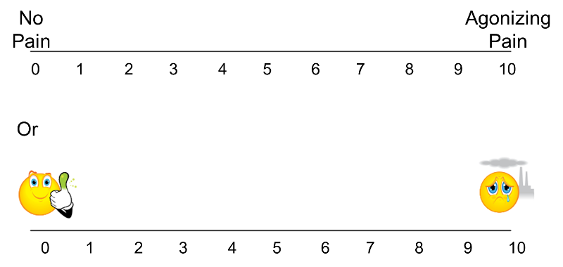
In the upper portion of the figure, certainly 10 is worse than 9, which is worse than 8; however, the difference between adjacent scores may not necessarily be the same. It is important to understand how outcomes are measured to make appropriate inferences based on statistical analysis and, in particular, not to overstate precision.
Assigning Ranks
The nonparametric procedures that we describe here follow the same general procedure. The outcome variable (ordinal, interval or continuous) is ranked from lowest to highest and the analysis focuses on the ranks as opposed to the measured or raw values. For example, suppose we measure self-reported pain using a visual analog scale with anchors at 0 (no pain) and 10 (agonizing pain) and record the following in a sample of n=6 participants:
7 5 9 3 0 2
The ranks, which are used to perform a nonparametric test, are assigned as follows: First, the data are ordered from smallest to largest. The lowest value is then assigned a rank of 1, the next lowest a rank of 2 and so on. The largest value is assigned a rank of n (in this example, n=6). The observed data and corresponding ranks are shown below:
|
Ordered Observed Data: |
0 |
2 |
3 |
5 |
7 |
9 |
|
Ranks: |
1 |
2 |
3 |
4 |
5 |
6 |
A complicating issue that arises when assigning ranks occurs when there are ties in the sample (i.e., the same values are measured in two or more participants). For example, suppose that the following data are observed in our sample of n=6:
Observed Data: 7 7 9 3 0 2
The 4th and 5th ordered values are both equal to 7. When assigning ranks, the recommended procedure is to assign the mean rank of 4.5 to each (i.e. the mean of 4 and 5), as follows:
|
Ordered Observed Data: |
0.5 |
2.5 |
3.5 |
7 |
7 |
9 |
|
Ranks: |
1.5 |
2.5 |
3.5 |
4.5 |
4.5 |
6 |
Suppose that there are three values of 7. In this case, we assign a rank of 5 (the mean of 4, 5 and 6) to the 4th, 5th and 6th values, as follows:
|
Ordered Observed Data: |
0 |
2 |
3 |
7 |
7 |
7 |
|
Ranks: |
1 |
2 |
3 |
5 |
5 |
5 |
Using this approach of assigning the mean rank when there are ties ensures that the sum of the ranks is the same in each sample (for example, 1+2+3+4+5+6=21, 1+2+3+4.5+4.5+6=21 and 1+2+3+5+5+5=21). Using this approach, the sum of the ranks will always equal n(n+1)/2. When conducting nonparametric tests, it is useful to check the sum of the ranks before proceeding with the analysis.
To conduct nonparametric tests, we again follow the five-step approach outlined in the modules on hypothesis testing.
- Set up hypotheses and select the level of significance α. Analogous to parametric testing, the research hypothesis can be one- or two- sided (one- or two-tailed), depending on the research question of interest.
- Select the appropriate test statistic. The test statistic is a single number that summarizes the sample information. In nonparametric tests, the observed data is converted into ranks and then the ranks are summarized into a test statistic.
- Set up decision rule. The decision rule is a statement that tells under what circumstances to reject the null hypothesis. Note that in some nonparametric tests we reject H0 if the test statistic is large, while in others we reject H0 if the test statistic is small. We make the distinction as we describe the different tests.
- Compute the test statistic. Here we compute the test statistic by summarizing the ranks into the test statistic identified in Step 2.
- Conclusion. The final conclusion is made by comparing the test statistic (which is a summary of the information observed in the sample) to the decision rule. The final conclusion is either to reject the null hypothesis (because it is very unlikely to observe the sample data if the null hypothesis is true) or not to reject the null hypothesis (because the sample data are not very unlikely if the null hypothesis is true).